Business Intelligence
Anomaly Detection for Business Metrics: A Practical Guide
A practical workflow to detect and investigate metric anomalies: baselines, seasonality, thresholds, backtesting, and governed audits.

I treat a metric alert as a reason to investigate - not proof that something went wrong. My starting point: define the metric, check that the data is complete, and compare results with similar periods - not just a business target.
For example, 4.8% conversion means 48 purchases out of 1,000 eligible visitors. Whether that deserves an alert depends on past rates, visitor counts, and normal weekday patterns.
Here’s the workflow I use:
- Define the inputs: Agree on calculations, reporting dates, exclusions, and ownership.
- Set the baseline: Account for trends, seasonality, and normal variation.
- Test the rules: Choose thresholds and volume limits, then measure false alerts, missed incidents, and detection delay without using future data.
- Check the cause: Review data errors, related metrics, and affected customer groups before escalating.
- Keep an audit trail: Save queries, settings, and decisions so others can check the result.
I start with one metric and one owner, then run alerts in shadow mode for two to four weeks. The goal is an alert your team can verify and act on - not another dashboard warning.
::: @figure 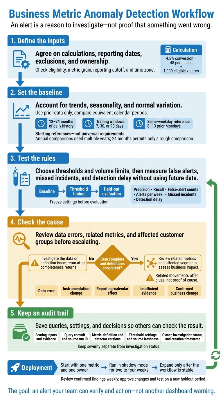 {Business Metric Anomaly Detection Workflow}
:::
{Business Metric Anomaly Detection Workflow}
:::
SREcon17 Asia/Australia: Smart Monitoring System for Anomaly Detection on Business Trends in Alibaba
::: @iframe https://www.youtube.com/embed/IUFuoqUPwPE :::
Build Baselines for Trends and Seasonality
Once the metric definition is fixed, build a baseline that reflects normal variation.
Start with 12–24 months of daily data, with one row per date in daily_metrics. Include metric_date, revenue_usd, conversions, eligible_visitors, customers_churned, customers_at_start, plan, and acquisition_channel. Add calendar flags for holidays, weekday, fiscal period, and daylight-saving transitions. [4]
Calculate Rolling Means and Median Baselines
Choose the window before the threshold. A rolling mean responds quickly but is sensitive to spikes. A rolling median and MAD resist isolated extremes. Calculate MAD against the median of the same window - not each historical day’s own rolling median. Require as many valid prior observations as the window length. [3]
| Trailing window | Useful starting point | Main limitation |
|---|---|---|
| 7 days | Fast daily monitoring with seven valid prior days | Does not adjust for weekday effects on its own |
| 30 days | Volatile metrics with about a month of history | Can lag after a sustained change |
| 90 days | Noisy metrics needing a steadier reference | Can miss recent growth or structural shifts |
After confirming the metric grain, use the same window logic for revenue, conversion, and churn. This PostgreSQL example builds a baseline from historical warehouse data and shows the intermediate calculations.
WITH baselines AS (
  SELECT
    d.metric_date,
    d.revenue_usd,
    h.valid_days,
    h.mean_7d,
    h.sd_7d,
    m.median_7d,
    a.mad_7d
  FROM daily_metrics AS d
  CROSS JOIN LATERAL (
    SELECT
      COUNT(revenue_usd) AS valid_days,
      ARRAY_AGG(revenue_usd)
        FILTER (WHERE revenue_usd IS NOT NULL) AS values_7d,
      AVG(revenue_usd) AS mean_7d,
      STDDEV_SAMP(revenue_usd) AS sd_7d
    FROM daily_metrics
    WHERE metric_date >= d.metric_date - INTERVAL '7 days'
      AND metric_date < d.metric_date
  ) AS h
  CROSS JOIN LATERAL (
    SELECT
      PERCENTILE_CONT(0.5) WITHIN GROUP (
        ORDER BY v
      ) AS median_7d
    FROM UNNEST(h.values_7d) AS values_in_window(v)
  ) AS m
  CROSS JOIN LATERAL (
    SELECT
      PERCENTILE_CONT(0.5) WITHIN GROUP (
        ORDER BY ABS(v - m.median_7d)
      ) AS mad_7d
    FROM UNNEST(h.values_7d) AS values_in_window(v)
  ) AS a
)
SELECT
  metric_date,
  revenue_usd,
  CASE WHEN valid_days = 7 THEN mean_7d END AS mean_7d,
  CASE WHEN valid_days = 7 THEN sd_7d END AS sd_7d,
  CASE WHEN valid_days = 7 THEN median_7d END AS median_7d,
  CASE WHEN valid_days = 7 THEN mad_7d END AS mad_7d,
  -- NULL means insufficient history or undefined due to zero variation.
  CASE WHEN valid_days = 7 THEN
    (revenue_usd - mean_7d) / NULLIF(sd_7d, 0)
  END AS z_score_7d,
  CASE WHEN valid_days = 7 THEN
    (revenue_usd - median_7d) / NULLIF(1.4826 * mad_7d, 0)
  END AS robust_z_score_7d
FROM baselines
ORDER BY metric_date;
Adjust the percentile syntax for your database engine.
Account for Seasonality and Trends
Match the baseline to your business rhythm. Compare Mondays with prior Mondays, not the previous day, using 8–13 prior Mondays as the reference. Annual comparisons need multiple years of history; 24 months allows only a rough comparison.
Treat holiday Mondays, quarter-end periods, and fiscal calendars separately. Handle daylight-saving transitions in the reporting time zone so duplicate or missing local hours don’t trigger alerts.
For growing revenue, statsmodels STL separates trend, weekly seasonality, and residual variation. In production, fit the model only on information available before the date being scored. [5][6] Use these baselines as the reference for detection rules and alert thresholds.
import pandas as pd
from statsmodels.tsa.seasonal import STL

df = (
    daily_metrics
    .sort_values("metric_date")
    .set_index("metric_date")
    .asfreq("D")
)

series = df["revenue_usd"].interpolate(limit=2)

stl = STL(
    series,
    period=7,          # daily data with weekly seasonality
    robust=True
).fit()

df["trend"] = stl.trend
df["seasonal"] = stl.seasonal
df["residual"] = stl.resid

residual_median = df["residual"].rolling(
    30, min_periods=14
).median().shift(1)

residual_mad = (
    df["residual"]
    .sub(residual_median)
    .abs()
    .rolling(30, min_periods=14)
    .median()
    .shift(1)
)

df["robust_residual_score"] = (
    df["residual"] - residual_median
) / (1.4826 * residual_mad)

df["anomaly"] = df["robust_residual_score"].abs() >= 3.5
If you interpolate small gaps, keep a separate data-quality check so a true outage still shows up.
Calculate Revenue, Conversion, and Churn Examples
Revenue: Daily revenue of $125,400.00, a prior-seven-day mean of $100,000.00, and sample standard deviation of $8,000.00 give
(125,400 − 100,000) ÷ 8,000 = 3.175. A median of $98,000.00 and MAD of $5,000.00 give a robust score of approximately 3.69. Both exceed example thresholds of 3 and 3.5.Conversion: On October 4, 2026, 48 conversions ÷ 1,000 eligible visitors = 4.8%. Use comparable eligibility rules, attribution windows, and dates; calculate historical rates as
SUM(conversions) ÷ SUM(eligible_visitors), not an average of percentages. Suppress alerts below 100 eligible visitors as a starting guard.Churn: For September logo churn, 12 cancellations ÷ 240 customers active and paying on September 1, 2026 = 5.0%; exclude later joiners from the cohort. Suppress alerts below 30 eligible customers as a starting guard. [4]
Compare plan and acquisition-channel segments with their own history. When counts stay sparse, aggregate over a longer period. [4]
Choose Detection Rules and Reduce False Alerts
A statistical anomaly doesn’t always call for action. Build the baseline, choose a detection rule, then backtest it. Set thresholds based on the metric’s historical volatility, the cost of missing an incident, and how many alerts the team can investigate. If a rule generates 100 alerts per week but the team can review only 10, it won’t help. Escalate changes that need action and log the rest.
Compare Detection Methods
Use the baseline from the previous section to choose the simplest rule that fits the metric’s cadence and noise.
| Method | Assumption and suitable metrics | Strength | Weakness | Typical false-alert pattern |
|---|---|---|---|---|
| Fixed thresholds | Known business limits; revenue floors and SLA metrics | Simple and tied to policy | Ignores scale changes and seasonality | Noisy when normal ranges change |
| Prior-period comparison | Previous period represents normal behavior; stable daily revenue or traffic | Easy to explain | Unusual prior periods distort comparisons | Noisy around weekends and promotions |
| Same-weekday or prior-year comparison | Comparable calendar patterns; revenue, visits, conversion, and retail demand | Accounts for recurring patterns | Pricing changes and holidays weaken comparisons | Less noisy with stable seasonality |
| Rolling z-score | Stable recent mean and variance; high-volume metrics | Fast and easy to interpret | Outliers and variance changes distort thresholds | Clustered alerts during shifts |
| Rolling median and MAD | Median and robust spread describe normal behavior; bursty revenue and orders | Resists isolated outliers | Can lag gradual changes; MAD may be zero | Fewer outlier-driven false alerts |
| Seasonal decomposition | Separable trend and seasonality; daily or hourly metrics | Makes recurring effects explicit | Needs enough history; struggles with structural breaks | Less noise with stable seasonality; more around unusual holidays |
| EWMA or control charts | Stable process baseline; conversion and operational rates | EWMA detects gradual shifts; Shewhart charts detect abrupt changes | Requires tuned limits and stable baselines | Repeated alerts during sustained shifts |
| Forecast-based detection | Expected values and uncertainty can be estimated; revenue and demand | Handles trend and multiple seasonal effects | Harder to maintain and validate | Depends on interval calibration; structural changes increase noise |
These are qualitative expectations, not measured rankings. NIST notes that EWMA gives older observations less weight. Its weighting factor controls sensitivity to gradual changes. Values around 0.15 to 0.30 are commonly suggested for small shifts, but choose the value through backtesting rather than using a default.[8][9]
Set Minimum Volumes and Alert Severity
Rate alerts need uncertainty estimates that account for the denominator. Set minimum eligible-user and customer counts using historical volume, acceptable uncertainty, and the cost of missed incidents - not a universal cutoff. Below that minimum, log or downgrade the signal, aggregate over longer periods, and use binomial confidence intervals or a suitable rate model.
Define severity by magnitude, duration, direction, and segment impact. For noisy demand metrics, require persistence - for example, two consecutive breaches. Allow faster escalation for payment failures or clear customer harm.
Group related alerts within a set correlation window, such as 60 minutes. During a cooldown, let repeat breaches update the existing incident instead of creating another one. Set recovery and reopening rules, too. Persistence cuts interruptions, but it also delays detection and can miss short incidents.
Backtest Rules Without Future Data
Test the rule on historical periods before deployment. In Snowflake, BigQuery, Redshift, or Postgres, split the history into baseline, threshold-tuning, and later held-out evaluation windows. Fix those window boundaries so the benchmark can be reproduced.
Tune thresholds, volume guards, persistence, and cooldowns only in the tuning window, then freeze them before evaluation. Keep the data in time order. Use only data available before the alert timestamp, excluding future values and later corrections. Document metric definitions, missing-data handling, parameters, and incident start and end times. Record whether each incident was a data error or a business change.
Report precision, recall, false-alert counts, alerts per week, missed incidents, and detection delay. Period-level scoring counts each hour or day; incident-level scoring counts each episode once within a predefined tolerance.[7][10]
Compare one-period and persistent rules on the same held-out window. Report detection delays and missed short incidents - not just the drop in alert counts. Review unmatched alerts before calling them false positives, since incomplete incident labels can distort scores.
Next, check each alert against data quality checks and related metrics before escalation.
Validate Data and Investigate Changes
Check the data, review neighboring metrics, then publish the reason for the change.
Check Data Quality and Metric Definitions
An alert is a prompt to check the data - not proof of a business change. Start with the cutoff, time zone, partition arrival, row counts, duplicate keys, nulls, schema changes, and joins. Make sure the numerator and denominator use the same eligible population. Review ingestion jobs, warehouse tasks, backfills, and dbt changes. dbt’s not_null, unique, accepted_values, and relationships tests can help spot structural failures.[11][12][15][16] Use the detector’s alert inputs to distinguish pipeline failures, definition shifts, and actual business changes.
Build a calendar-and-segment spine, then left join observations. Assign observation_status as missing, null_value, true_zero, or observed. Even a true zero needs a completeness check. Review the governed metric definition, too: a query can run without errors and still measure the wrong thing.[13][14]
The matrix below links each detector flag to a likely failure mode. Use it to decide whether you’re dealing with a data issue, a definition issue, or an actual metric move.
| Symptom | Evidence to check | Response |
|---|---|---|
| Missing observation | No row for an expected period or segment | Investigate coverage; do not impute zero |
| Sparse metric | Small denominator or many unavailable values | Report coverage; aggregate only if allowed |
| Definition shift | Changed filters, grain, joins, or dbt logic | Reconcile definitions over an overlap period |
| Holiday, billing-cycle, or cutoff shift | Holiday, billing-cycle position, or reporting cutoff differs | Compare equivalent calendar periods |
| Isolated outlier | Duplicate key, unusual transaction, refund, or join multiplication | Inspect contributing records; keep valid transactions |
| Late-arriving data | Late partition, failed task, retry, or unfinished backfill | Escalate to the data owner; rerun after completeness returns |
Once the data checks pass, review adjacent metrics and segments to find where the change first appears.
Investigate Related Metrics and Segments
Trace revenue through invoices, payments, refunds, chargebacks, and failures. For conversion, follow traffic through checkout and purchase. For churn, review renewals, cancellations, and active-customer counts to understand retention trends.
Compare affected and unaffected groups using approved dimensions such as plan, channel, region, device, or customer cohort. Before deciding that performance declined, check whether the customer mix changed. Related movements offer clues, not proof of cause.
Show the Calculation and Reason
Show the calculation, not just the alert. Display the inputs and explain why the alert fired. Keep the scoring logic open to review so analysts can check the same inputs in Snowflake, BigQuery, Redshift, or Postgres.
This Postgres SQL shows the bounds, deviation, score, and alert reason. Check data-quality status before business-alert conditions, and handle zero or missing spread explicitly instead of dividing by zero.
WITH scored AS (
  SELECT *,
    expected_value - baseline_spread AS lower_bound,
    expected_value + baseline_spread AS upper_bound,
    actual_value - expected_value AS deviation,
    (actual_value - expected_value)
      / NULLIF(baseline_spread, 0) AS score
  FROM metric_alert_inputs
)
SELECT metric, segment, timestamp,
       actual_value, expected_value,
       lower_bound, upper_bound, deviation, score,
       CASE
         WHEN data_quality_status IS DISTINCT FROM 'passed'
           THEN 'pipeline_stale'
         WHEN actual_value IS NULL THEN 'missing_observation'
         WHEN minimum_volume_met IS DISTINCT FROM TRUE
           THEN 'low_denominator'
         WHEN actual_value < lower_bound THEN 'below_lower_bound'
         WHEN actual_value > upper_bound THEN 'above_upper_bound'
         ELSE 'within_bounds'
       END AS alert_reason
FROM scored;
Use the same precedence in Python. Keep both SQL and Python editable, with identical precedence. When porting to Snowflake, BigQuery, or Redshift, verify timestamp arithmetic, null handling, and window-function behavior.
Store the scoring inputs, classification, and evidence so every alert can be reproduced. Include the query commit, threshold settings, source run ID, metric-definition and detector versions, source freshness, investigation status, owner, and creation timestamp.
Keep severity separate from investigation status. An urgent data issue, such as a stale pipeline, isn’t a confirmed business change. Record the final classification as data error, instrumentation change, reporting-calendar effect, insufficient evidence, or confirmed business change.
Run and Evaluate a Governed Workflow
After backtesting, put the rule into a governed workflow and publish a benchmark that others can rerun.
Run Governed Investigations in Querio
Before enabling detection, assign one metric owner, one backup investigator, and one Slack or email destination. Schedule runs after the data-availability cutoff. Link the source query, detection result, and decision so each investigation has an audit trail.
Use Slack or email for delivery only. Querio supports live, read-only warehouse connections, plus inspectable and editable SQL and Python in editable notebooks that rerun when data changes. Keep metric definitions, calendars, exclusions, ownership, and procedures in version-controlled context files alongside dbt models. Require human approval for changes.
Role-based self-serve access lets analysts investigate within their permissions. Scheduled investigations can send concise findings through Slack or email. Store outcomes in a governed audit table - not ad hoc warehouse tables. This setup also keeps the evidence needed to evaluate rule quality.[1]
Once alerts are routed and audited, compare rules on the same metric using a frozen dataset.
Publish a Reproducible Detection Benchmark
Publish executable results, not manually entered scores. This synthetic conversion-rate benchmark uses seed 42, daily binomial counts, trend, weekly seasonality, and labeled injected anomalies. Tune on normal days in 2024, then evaluate on 2025–2026 data.
The benchmark measures business-alert quality - false alerts, recall, and delay - not model accuracy. The code generates the Markdown comparison table. Results are illustrative, not customer outcomes.
# Reproduction environment: Python 3.11,
# numpy==1.26.4, pandas==2.2.3
import numpy as np
import pandas as pd

rng = np.random.default_rng(42)
dates = pd.date_range("2024-01-01", "2026-09-30")
t = np.arange(len(dates))
volume = rng.poisson(2000, len(dates))
probability = (
    0.12 + 0.000015 * t
    + 0.012 * np.sin(2 * np.pi * dates.dayofweek.to_numpy() / 7)
)

injected = pd.to_datetime([
    "2024-04-15", "2024-08-20", "2024-11-12",
    "2025-02-10", "2025-06-17", "2025-10-08",
    "2026-01-19", "2026-05-12", "2026-09-09"
])
label = pd.Series(dates.isin(injected), index=dates)
probability[label.to_numpy()] *= 0.65
purchases = rng.binomial(volume, probability)
rate = pd.Series(purchases / volume, index=dates)

# Save the exact inputs and labels with the benchmark.
pd.DataFrame({
    "sessions": volume, "purchases": purchases,
    "conversion_rate": rate, "injected_anomaly": label
}, index=dates).to_csv("synthetic_conversion.csv", index_label="date")

baselines = {
    "28-day mean": rate.shift(1).rolling(28).mean(),
    "28-day median": rate.shift(1).rolling(28).median(),
    "8-week same-weekday mean": pd.concat(
        [rate.shift(7 * k) for k in range(1, 9)], axis=1
    ).mean(axis=1, skipna=False)
}
eligible = pd.Series(volume >= 1000, index=dates)
tuning = pd.Series(
    (dates >= "2024-01-01") & (dates <= "2024-12-31"),
    index=dates
)
evaluation = pd.Series(
    (dates >= "2025-01-01") & (dates <= "2026-09-30"),
    index=dates
)

print("Tuning: Jan. 1–Dec. 31, 2024; evaluation: "
      "Jan. 1, 2025–Sept. 30, 2026.")
print("Unit: one alert per metric-day; minimum sessions: 1,000.")
print("Delay: days from injected event to detection; "
      "delivery latency excluded.")
headers = [
    "Baseline", "Threshold (pp)", "Eligible days", "Actual anomalies",
    "Detections", "TP", "FP", "FN", "TN",
    "False-alert rate", "Recall", "Median delay"
]
print("| " + " | ".join(headers) + " |")
print("| " + " | ".join(["---"] * len(headers)) + " |")

for name, baseline in baselines.items():
    deviation = (rate - baseline).abs()
    ready = eligible & baseline.notna()
    threshold = deviation[tuning & ready & ~label].quantile(0.99)
    test = evaluation & ready
    alert = (deviation > threshold) & test
    positive = label & test
    negative = ~label & test
    tp = int((alert & positive).sum())
    fp = int((alert & negative).sum())
    fn = int((~alert & positive).sum())
    tn = int((~alert & negative).sum())
    normal_days = int(negative.sum())
    actual = int(positive.sum())
    row = [
        name, f"{threshold * 100:.3f}", str(int(test.sum())),
        str(actual), str(int(alert.sum())), str(tp), str(fp),
        str(fn), str(tn),
        f"{fp}/{normal_days} = {fp / normal_days:.2%}",
        f"{tp}/{actual} = {tp / actual:.1%}",
        "0 days" if tp else "N/A"
    ]
    print("| " + " | ".join(row) + " |")
The injected anomalies last one day, so this benchmark does not test persistent incidents or notification latency. Save the code commit and dependency versions with the results.
Review confirmed findings weekly. Then propose rule changes for owner approval and test them on a new holdout period - not the evaluation window you've already inspected.
Start with One Metric First
With the workflow and benchmark in place, choose one high-value metric and one accountable owner before expanding coverage. Approve the metric's definition, use the seasonal baseline you've already validated, validate inputs, and backtest thresholds.
Run in shadow mode for two to four weeks before routing actionable alerts. Record investigation outcomes, and expand only after the workflow is stable.[17][18][19]
FAQs
::: faq
How can I detect anomalies with limited historical data?
Build baselines that account for context. Standardize reporting intervals, identify missing data, and stabilize variance. Compare metrics from similar hours, weekdays, or seasons using rolling medians and median absolute deviation (MAD), or lagged baselines - not a global average.
When historical data is limited or behavior changes fast, use simple, explainable thresholds on residuals - the differences between observed values and the baseline. Group adjacent flagged points for review, calibrate thresholds using a representative deployment window, and record scores, baselines, and decision metadata [1][2]. :::
::: faq
When should I reset a baseline after a business change?
Reset or rebuild your anomaly baseline when a business change shifts what “normal” looks like. Triggers include a product or feature launch, a metric definition change, a pipeline or schema change, a time zone or ingestion shift, major data corrections, or evidence of drift in feature or score distributions. After major data corrections, backfill and replay.
Don’t reset out of habit. Retrain based on reviewed evidence, compare the candidate baseline or model using the same replay windows, and set rollback conditions before switching. [1] :::
::: faq
How do I limit false alerts across many segments?
Calibrate thresholds using an evaluation set that matches deployment conditions and your team’s capacity to respond. Then test across multiple time windows and series [1]. Group adjacent flagged points into events and remove duplicate notifications [1].
Use dynamic thresholds that account for seasonality and context, such as Z-scores or IQR, instead of static cutoffs [2]. Send low-confidence anomalies to a review queue. Record supporting evidence - including thresholds, versions, and review outcomes - to guide further tuning [1]. :::