Window Functions SQL: The Complete Analyst's Guide

Your CEO asks for a quick report before the Monday standup: top three salespeople by revenue in each region, plus each person’s share of regional revenue, plus whether they moved up or down from last quarter.

You can answer that with basic SQL. But if you only reach for GROUP BY, the query often becomes awkward. You summarize the data, lose the row-level detail, then build it back with joins, nested subqueries, or spreadsheet cleanup.

That is the pain point window functions sql solves.

Window functions let you calculate across a related set of rows while keeping every original row visible. You can rank reps inside each region, compute running totals by day, compare each month to the prior month, or build retention views without flattening the dataset into one row per group. The result feels less like report-writing and more like analysis.

For product managers and junior analysts, this changes the kind of questions you can answer directly in the warehouse. For data teams, it reduces the need to keep rebuilding the same “top N,” “change vs previous period,” and “rolling average” logic in dashboards and notebooks.

The Analytical Superpower Hiding in Your SQL

A lot of teams first meet window functions when a report becomes a little too specific for GROUP BY.

Take a regional sales report. A product leader does not want total revenue by region. They want each salesperson listed, their revenue, their rank within region, and the gap from the rep above them. That is where standard aggregation starts fighting you.

With GROUP BY, you can get this:

• one row per region

• one row per salesperson

• one row per quarter

You cannot get all three views at once in a single clean result without extra work.

Why GROUP BY starts to break down

GROUP BY is built to collapse rows. That is useful when you want a summary table. It is frustrating when you want a summary alongside the original records.

A junior analyst often writes a query like this:

SELECT
  region,
  salesperson,
  SUM(revenue) AS revenue
FROM sales
WHERE order_date >= '2024-10-01'
  AND order_date < '2025-01-01'
GROUP BY region, salesperson;

That part is fine. The trouble starts when someone asks, “Which three people were the top performers in each region?”

Now you need ranking logic per region. Then someone asks, “Add each person’s share of total regional revenue.” Then, “Show last quarter too so I can compare movement.”

At that point, the query often turns into a stack of subqueries.

What window functions change

Window functions let you keep each salesperson row and compute extra analytical values around it.

You can:

• rank rows inside each region

• compare a row to the prior row

• compute a cumulative total over time

• pull first or last values inside a group

The key idea is simple. A window function looks at a set of related rows, but it does not merge them into one output row.

Practical takeaway: Use GROUP BY when you want fewer rows. Use a window function when you want the same rows plus more context.

That is why window functions feel like an analytical superpower. They preserve detail while adding summary logic. For self-serve reporting, that matters because product managers and operators usually need both at once.

Understanding the Window and Its Core Syntax

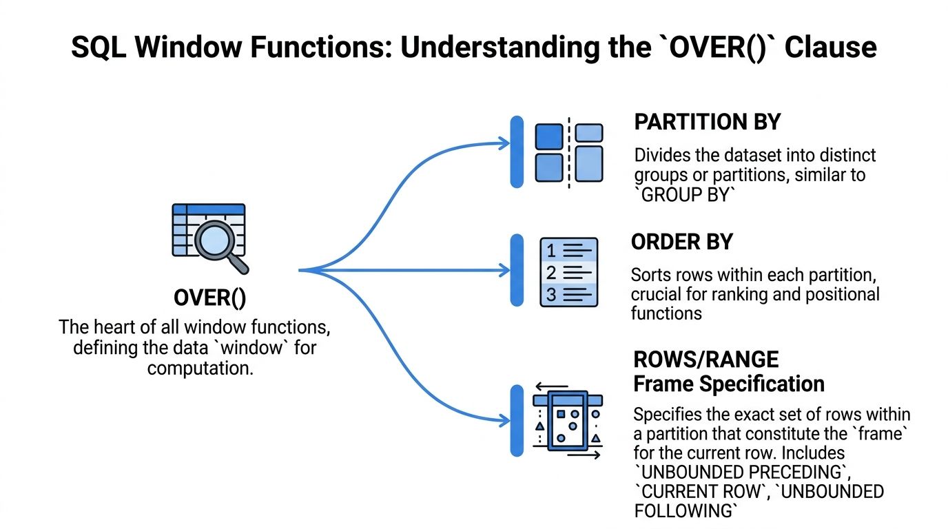
Every window function depends on one construct: OVER().

That clause tells SQL which rows belong to the calculation for the current row. If the function is the math, OVER() is the rulebook.

Think in lanes and finish order

Use a race analogy.

• PARTITION BY puts runners into separate lanes or race groups.

• ORDER BY arranges runners inside each lane by finish order.

• Later, ROWS or RANGE narrows the exact slice of rows used for each calculation.

If you partition by region, each region becomes its own mini-dataset. If you then order by revenue DESC, SQL can rank reps from highest to lowest inside each region.

The simplest shape of a window function

function_name(...) OVER (
  PARTITION BY ...
  ORDER BY ...
)

A basic ranking example:

SELECT
  region,
  salesperson,
  revenue,
  ROW_NUMBER() OVER (
    PARTITION BY region
    ORDER BY revenue DESC
  ) AS sales_rank
FROM sales_summary;

This returns every row plus a rank number inside each region.

What PARTITION BY really does

PARTITION BY splits the dataset into groups for calculation, but unlike GROUP BY, it does not reduce the result set.

If you remove PARTITION BY, the function sees the whole result as one group.

Compare these two ideas:

That single change often determines whether a report answers the business question correctly.

What ORDER BY inside OVER() controls

This ORDER BY is not the same as the final output ordering of the query.

Inside a window function, it defines the sequence used for ranking, lagging, leading, and running calculations. Without the right sequence, the result can be meaningless.

For example, if you want month-over-month change, you need rows ordered by month. If you want a sales leaderboard, you need rows ordered by revenue.

Why this became such an important SQL feature

Window functions were introduced in the ANSI SQL:2003 standard. Early commercial implementation arrived in SQL Server in the mid-2000s, supporting a limited set of ranking and aggregate functions. Later versions, like SQL Server in the early 2010s, expanded functionality to include frame specifications with ROWS and RANGE along with more analytic functions such as LAG and LEAD, helping to establish them as core tools in modern warehousing and BI work, as described in Redgate’s history of T-SQL window function performance.

If you want a grounding in standard reporting patterns before you layer in windows, this guide to top SQL queries for analytics is a useful companion.

Tip: When a result looks wrong, inspect the PARTITION BY first, then the ORDER BY. Most window-function mistakes come from defining the window incorrectly, not from choosing the wrong function.

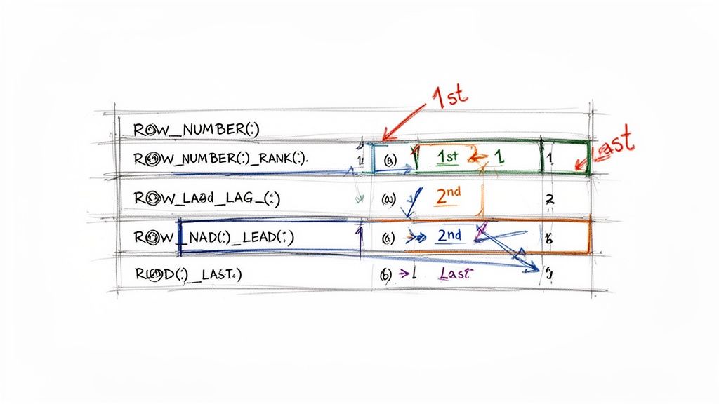
Essential Ranking and Positional Functions Explained

The fastest way to understand window functions is to compare similar functions on the same dataset.

Say you have this regional sales summary:

The tied values are useful because ties are exactly where analysts get tripped up.

Ranking functions side by side

Use this query:

SELECT
  region,
  salesperson,
  revenue,
  ROW_NUMBER() OVER (
    PARTITION BY region
    ORDER BY revenue DESC
  ) AS row_num,
  RANK() OVER (
    PARTITION BY region
    ORDER BY revenue DESC
  ) AS sales_rank,
  DENSE_RANK() OVER (
    PARTITION BY region
    ORDER BY revenue DESC
  ) AS dense_sales_rank
FROM sales_summary;

Here is how they differ:

In the East region:

• Ava and Ben tie on revenue.

• ROW_NUMBER() gives them different numbers.

• RANK() might give them both 1, then Chloe gets 3.

• DENSE_RANK() might give them both 1, then Chloe gets 2.

Which ranking function should you choose

This is usually a business decision, not a technical one.

Use ROW_NUMBER() when you need a single winner even if the data ties. That happens when deduplicating records or choosing the latest order per customer.

Use RANK() when a true tie should remain a tie. This works for “top performers” reporting.

Use DENSE_RANK() when stakeholders expect rank values without gaps. That is common in customer segmentation or prize tiers.

Key takeaway: If you are filtering to “top 3 by group,” check how ties should work before you write the SQL. The wrong ranking function can create the wrong business answer.

Positional functions for before and after comparisons

Ranking tells you where a row stands. Positional functions tell you what came before or after.

The most common are:

• LAG()

• LEAD()

• FIRST_VALUE()

• LAST_VALUE()

A monthly revenue example:

SELECT
  month,
  revenue,
  LAG(revenue) OVER (ORDER BY month) AS prior_month_revenue,
  LEAD(revenue) OVER (ORDER BY month) AS next_month_revenue
FROM monthly_revenue;

This pattern is perfect for period-over-period analysis.

You can then calculate change:

SELECT
  month,
  revenue,
  LAG(revenue) OVER (ORDER BY month) AS prior_month_revenue,
  revenue - LAG(revenue) OVER (ORDER BY month) AS absolute_change
FROM monthly_revenue;

For product teams, this supports questions like:

• Did weekly active users rise or fall from the prior week?

• Did conversion improve after a release?

• Which month broke a declining trend?

FIRST_VALUE() and LAST_VALUE() in practice

These functions pull a value from the beginning or end of a partition.

Example:

SELECT
  customer_id,
  order_date,
  order_value,
  FIRST_VALUE(order_value) OVER (
    PARTITION BY customer_id
    ORDER BY order_date
  ) AS first_order_value
FROM orders;

That is useful when you want to compare current behavior to a customer’s initial purchase, first subscription plan, or first recorded lifecycle stage.

LAST_VALUE() is where readers get confused. It depends on the window frame, not just the ordering. If you use it, it may return the current row’s value instead of the final value in the full partition.

When you want the final value in a partition, specify the frame explicitly.

SELECT
  customer_id,
  order_date,
  order_value,
  LAST_VALUE(order_value) OVER (
    PARTITION BY customer_id
    ORDER BY order_date
    ROWS BETWEEN UNBOUNDED PRECEDING AND UNBOUNDED FOLLOWING
  ) AS latest_order_value
FROM orders;

A practical leaderboard query

This is the kind of query product managers ask for:

WITH ranked_sales AS (
  SELECT
    region,
    salesperson,
    revenue,
    RANK() OVER (
      PARTITION BY region
      ORDER BY revenue DESC
    ) AS sales_rank
  FROM sales_summary
)
SELECT *
FROM ranked_sales
WHERE sales_rank <= 3;

That gives a top-three-per-region report without self-joins. It also leaves room to add more columns later, such as share of regional total or previous-quarter movement.

Aggregates Unleashed Running Totals and Moving Averages

Most analysts first use window functions for ranking. A significant advancement occurs when you apply aggregate functions like SUM() or AVG() without collapsing the rows.

That is where trend reporting gets easier.

Running totals without losing daily detail

Suppose you have daily revenue:

A running total is simple with a window aggregate:

SELECT
  date,
  revenue,
  SUM(revenue) OVER (
    ORDER BY date
    ROWS BETWEEN UNBOUNDED PRECEDING AND CURRENT ROW
  ) AS running_revenue
FROM daily_revenue;

Each row keeps its daily revenue and also shows cumulative revenue up to that date.

That frame clause matters:

• UNBOUNDED PRECEDING means start at the first row in the ordered set.

• CURRENT ROW means end at this row.

Together, they create a cumulative window.

Benchmarks cited in ThoughtSpot’s guide note that for large datasets, window-function queries for running totals can be 30-50% faster than older approaches like correlated subqueries. The same guide explains that ROWS uses physical row offsets, while RANGE uses value-based logic, and RANGE can reduce computation by 20-40% on pre-sorted data with ties in some cases. Their examples are collected in this tutorial on SQL window functions.

Department averages that stay attached to each row

This is another common win.

If Finance has salaries of 50k, 50k, and 20k, the department average is 40k. If Sales has 30k and 20k, the average is 25k. Window functions let you display that average alongside every employee row instead of replacing the employee list with one row per department.

SELECT
  employee_name,
  department,
  salary,
  AVG(salary) OVER (
    PARTITION BY department
  ) AS department_avg_salary
FROM employees;

That pattern is useful for compensation analysis, account health scoring, support volume by agent, and quota attainment.

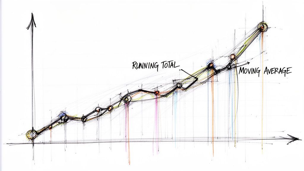
Moving averages with precise frames

A moving average is different from a running total because the window slides.

A classic example is a 7-day moving average:

SELECT
  date,
  revenue,
  AVG(revenue) OVER (
    ORDER BY date
    ROWS BETWEEN 6 PRECEDING AND CURRENT ROW
  ) AS revenue_7_day_ma
FROM daily_revenue;

This says: for each row, average the current row and the six rows before it.

For teams building growth dashboards, this smooths noisy daily swings and makes trend changes easier to interpret. If you work with product usage or subscription activity, this kind of pattern pairs well with broader time series analysis workflows.

A short visual helps here:

ROWS versus RANGE

This distinction matters more than most tutorials admit.

ROWS

ROWS counts physical row positions.

AVG(revenue) OVER (
  ORDER BY date
  ROWS BETWEEN 6 PRECEDING AND CURRENT ROW
)

That means exactly seven rows, assuming enough earlier rows exist.

RANGE

RANGE groups rows based on equal ordered values, not physical position.

If multiple rows share the same sort value, RANGE can include all tied rows together. That can be exactly right in some financial or pricing analyses, and very wrong in others.

Tip: For time-series business reporting, prefer ROWS when you need strict row counts. Reach for RANGE only when value-based grouping is intentional.

A practical pattern for percent of total

Window aggregates also solve “share of total” questions cleanly:

SELECT
  region,
  salesperson,
  revenue,
  revenue / SUM(revenue) OVER (PARTITION BY region) AS pct_of_region_revenue
FROM sales_summary;

That is one of the most useful self-serve reporting patterns in a warehouse. It lets every stakeholder see not just raw volume, but contribution.

Advanced Recipes for Modern Product Analytics

A single window function is useful. Several working together inside CTEs are where analysts start building durable reporting logic.

This is the point where syntax turns into a reusable analytical system.

Recipe one sessionizing product events

A raw event table often has one row per click, view, or API call. Product teams usually want sessions instead.

A common approach is:

1. Sort each user’s events by timestamp.

2. Use LAG() to look at the previous event time.

3. Flag a new session when the gap crosses your session threshold.

4. Use a cumulative sum to assign session numbers.

WITH ordered_events AS (
  SELECT
    user_id,
    event_time,
    event_name,
    LAG(event_time) OVER (
      PARTITION BY user_id
      ORDER BY event_time
    ) AS prior_event_time
  FROM events
),
session_flags AS (
  SELECT
    user_id,
    event_time,
    event_name,
    CASE
      WHEN prior_event_time IS NULL THEN 1
      WHEN event_time > prior_event_time THEN 0
      ELSE 0
    END AS new_session_flag
  FROM ordered_events
),
sessionized AS (
  SELECT
    user_id,
    event_time,
    event_name,
    SUM(new_session_flag) OVER (
      PARTITION BY user_id
      ORDER BY event_time
      ROWS BETWEEN UNBOUNDED PRECEDING AND CURRENT ROW
    ) AS session_id
  FROM session_flags
)
SELECT *
FROM sessionized;

The exact threshold logic depends on your warehouse and timestamp functions, but the core pattern remains the same. LAG() detects boundaries. A cumulative aggregate labels groups.

Recipe two cohort retention with CTEs

Retention analysis feels intimidating because you need a user’s first activity date and their later activity relative to that start.

A practical pattern is to define a first-touch row, then compare later rows to it.

WITH user_activity AS (
  SELECT
    user_id,
    activity_date
  FROM app_events
),
first_activity AS (
  SELECT
    user_id,
    MIN(activity_date) AS cohort_date
  FROM user_activity
  GROUP BY user_id
),
cohort_events AS (
  SELECT
    ua.user_id,
    fa.cohort_date,
    ua.activity_date,
    ROW_NUMBER() OVER (
      PARTITION BY ua.user_id
      ORDER BY ua.activity_date
    ) AS activity_sequence
  FROM user_activity ua
  JOIN first_activity fa
    ON ua.user_id = fa.user_id
)
SELECT *
FROM cohort_events;

ROW_NUMBER() helps when you need to distinguish first activity from later returns, or when you want to isolate the first event in each retention bucket.

The broader idea matters more than the exact SQL dialect. For retention work, combining window functions with CTEs is a common pattern. GeeksforGeeks notes that newer execution improvements such as PostgreSQL 17’s hybrid window execution reduced latency by up to 40% for multi-window queries, which makes these patterns more realistic for interactive reporting in self-serve environments. That discussion appears in their overview of window functions in SQL.

Practical advice: Build retention logic in layers. One CTE for cohort assignment, one for event ordering, one for aggregation. This makes debugging far easier than cramming everything into one giant query.

Recipe three year-over-year growth

Leadership teams ask for YoY metrics constantly. LAG() makes that pattern straightforward if your data is already summarized at the month or quarter level.

SELECT
  month,
  revenue,
  LAG(revenue, 12) OVER (
    ORDER BY month
  ) AS revenue_last_year,
  revenue - LAG(revenue, 12) OVER (
    ORDER BY month
  ) AS yoy_change
FROM monthly_revenue;

This compares each month to the same month one year earlier.

That is helpful for:

• board reporting

• pricing impact reviews

• seasonality analysis

• pipeline pacing checks

Recipe four self-serve leaderboards

Window functions become valuable when business users want reusable report patterns rather than one-off analyst work.

A clean leaderboard model often includes:

• revenue by rep

• rank within region

• share of regional total

• prior-period comparison

One way to support that in a modern stack is to keep the logic in warehouse-native SQL and expose the result in notebooks or analytics apps. Tools such as Hex, Looker, and Querio can sit on top of warehouse queries. Querio specifically runs AI coding agents directly on the warehouse using inspectable SQL and Python notebooks, which fits well when teams want natural-language access but still need advanced query patterns such as windows.

The SQL itself remains the durable asset. The interface just changes who can use it.

Mastering Performance Across Data Warehouses

A correct window function is not always a production-ready one.

The query that works on a sample table can become expensive on warehouse-scale event data, especially when partitions get huge or the ordering step forces heavy sorting.

Why performance gets tricky

Window functions often require the warehouse to sort data by the PARTITION BY and ORDER BY expressions before computing results. That means your query cost depends not only on the function you choose, but also on how much data sits inside each partition and how wide each row is.

On modern cloud warehouses, one of the most common mistakes is using a very large unbounded frame without thinking about the partition size. Chat2DB’s write-up notes that frames like ROWS BETWEEN UNBOUNDED PRECEDING AND CURRENT ROW can spike query costs by 10x on large partitions, which is why they frequently create production issues even though many beginner tutorials treat them as harmless defaults. Their examples are in this article on window-function performance tuning.

The biggest tuning levers

Partition choice

If you partition by a high-cardinality column, you may create many tiny groups. If you partition too broadly, you may create a few giant groups. Neither is automatically wrong, but both affect memory and execution.

Ask a simple question: does this partition match the business grain of the calculation?

• rank salespeople by region, not by the whole company

• compare events by user_id, not by a random surrogate dimension

• compute support queue trends by queue or team, not by an unnecessarily broad category

Ordering choice

Every ordered window needs a stable sort key. If the order column has ties and you do not break them, results can be non-deterministic for functions like ROW_NUMBER() and sometimes confusing for RANK() outputs.

A safer pattern is:

ROW_NUMBER() OVER (
  PARTITION BY region
  ORDER BY revenue DESC, salesperson ASC
)

That secondary sort key gives repeatable results.

Frame size

Many costs hide in frame size. A cumulative frame across a giant partition can be fine in one warehouse and expensive in another. A moving frame with a narrow boundary is often easier to reason about and sometimes cheaper to compute.

If the business question only needs a trailing period, define that period. Do not default to unbounded history.

Practical debugging checklist

When a window query feels slow or suspicious, work through this list:

• Check partition width: Are you grouping too much data together?

• Inspect sort keys: Are you ordering by a field with lots of ties or poor clustering?

• Trim selected columns: Wide intermediate rows add cost.

• Materialize earlier logic if needed: A pre-aggregated CTE or table can reduce rows before the window executes.

• Test with and without frame clauses: The default frame is not always what you think.

• Verify determinism: Add tie-breakers to ranking queries.

If you are troubleshooting slow warehouse SQL in general, this guide on optimizing a query is a good reference point.

Rule of thumb: Start with the smallest partition and narrowest frame that still answers the business question.

Warehouse-specific caution

Snowflake, BigQuery, Redshift, and Postgres all support window functions, but execution details differ. The syntax may look portable while the runtime behavior is not.

A few habits travel well across systems:

The biggest practical lesson is this: window functions are not just a syntax feature. They are a modeling choice. If your warehouse is paying a heavy price, revisit the shape of the analysis, not only the SQL text.

From Analyst Bottleneck to Self-Serve Powerhouse

Teams treat advanced SQL as a specialist skill reserved for the data team. Window functions challenge that habit.

Once you understand partitions, ordering, and frames, you can answer a wide range of business questions directly in the warehouse: top performers, retention, period-over-period change, rolling trends, contribution to totals, and more. Those are not edge cases. They are the everyday work of product, finance, and operations.

For teams trying to reduce reporting queues and make data access broader, the ultimate goal is not just better SQL. It is better infrastructure for decisions. That is the promise behind self-serve analytics.

If your team wants self-serve analysis without giving up warehouse-native SQL, Querio is one option to evaluate. It runs AI coding agents directly on your data warehouse and works with inspectable SQL and Python notebooks, which can help teams turn patterns like window functions into reusable analytics workflows for both technical and non-technical users.