Guide
Mastering Monte Carlo Simulations for Analytics 2026
Master Monte Carlo simulations for better decision-making in product analytics. Explore core concepts, use cases, and practical implementation.

You're probably dealing with a forecast that looks precise on the surface and shaky underneath. A new feature launch, a pricing change, a migration, a growth target. The spreadsheet asks for a single conversion rate, a single churn number, a single infrastructure cost. You type in your best guesses, knowing full well that reality won't cooperate.
That's the moment where many fall into false certainty. They ask, “What will happen?” when the honest question is, “What could happen, and how likely is each version?” Monte Carlo simulations are built for that second question. They replace a brittle average with a range of possible futures, then show you the shape of uncertainty instead of hiding it.
Table of Contents
- Beyond the Best Guess
- What Are Monte Carlo Simulations Really
- Why Your Business Needs This Method
- Avoiding the Garbage In Garbage Out Trap
- Practical Implementation in Your Analytics Workflow
- Scaling Simulations in a Modern Data Warehouse
- Validating and Trusting Your Results
Beyond the Best Guess
A product manager needs a launch forecast by Friday. Revenue depends on sign-up volume, activation rate, trial conversion, support load, and whether infra costs spike under heavier usage. Each input is uncertain, but the planning sheet wants one number in every cell.
So the team does what teams usually do. They pick a “most likely” value for each input, maybe add a best case and a worst case, and push the model forward. The final answer feels polished because it came from a spreadsheet. It still hides the thing leadership needs to know, which is uncertainty.
Monte Carlo simulations change the framing. Instead of saying “activation will be 18%” or “cloud cost will be this amount,” you describe plausible ranges and likelihoods. Then you let the computer sample from those assumptions again and again, building many possible versions of the future.
That shift matters because business outcomes are usually driven by combinations of uncertainty, not isolated variables. A slightly weaker conversion rate might be fine if adoption is strong. A modest delay might be harmless unless it overlaps with high support demand. What hurts teams isn't just being wrong on one input. It's being wrong on several at once and not seeing how they interact.
Monte Carlo is less about predicting one answer and more about stress-testing your thinking against many possible answers.
The practical payoff is better conversations. Instead of debating whose single estimate is “right,” you can ask better questions:
- How wide is the likely outcome range: Is this decision stable or fragile?
- What downside should we prepare for: Which bad outcomes are plausible enough to matter?
- Which inputs drive the spread: Where should we invest in better data or tighter controls?
For a smart product manager, that's the fundamental upgrade. You stop treating uncertainty as an embarrassment and start modeling it directly.
What Are Monte Carlo Simulations Really
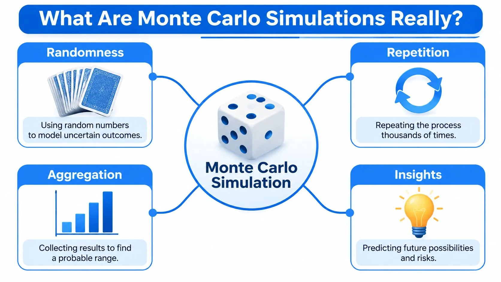
Monte Carlo simulations sound more intimidating than they are. At heart, they're repeated computational experiments under uncertainty.
The method itself has a serious pedigree. It was first conceived in 1946 by Stanisław Ulam at Los Alamos National Laboratory to calculate neutron diffusion paths for the hydrogen bomb, and Nick Metropolis named it after Monte Carlo because chance sat at the center of the process, as described in Los Alamos's history of the Monte Carlo method. But you don't need nuclear physics to understand the idea.
A simple mental model
Suppose you draw a weird shape on the floor and want its area. There's no easy formula. One workaround is to throw a huge number of tiny dots across the room at random and count how many land inside the shape. The fraction inside gives you an estimate of the area.
That's the basic logic behind Monte Carlo. When a system is too messy for neat closed-form math, you can often learn about it by random sampling and repetition.
If you've ever noticed that your intuition about uncertainty can be unreliable, this short read on why probability feels unintuitive in practice helps explain why Monte Carlo methods are so useful.
The three moving parts
A Monte Carlo simulation usually has three core ingredients.
-
Uncertain inputs as distributions
You don't feed the model a single value for each variable. You describe each variable as a range with a probability pattern. -
A model that connects inputs to outputs
This can be simple, like profit = revenue - cost, or much more involved. -
Repeated sampling
The computer draws random values from each input distribution, runs the model once, stores the outcome, and repeats the process many times.
After enough repetitions, the output stops looking like isolated guesses and starts looking like a distribution. That output distribution tells you more than any average can. You can inspect the center, the spread, the tail risks, and the likelihood of crossing a business threshold.
Here's the intuition in plain language:
| Component | What it means | Business translation |
|---|---|---|
| Randomness | Sample possible input values | Try one plausible future |
| Repetition | Run the model many times | Don't trust a single trial |
| Aggregation | Collect all outcomes | See the full range |
| Interpretation | Read the distribution | Make a risk-aware decision |
Practical rule: A Monte Carlo model is a machine for turning uncertainty in inputs into a probability distribution for outcomes.
That's all it is. Not magic. Not a black box by definition. Just disciplined repetition with uncertain inputs.
Why Your Business Needs This Method
Most business forecasts still rely on a narrow pattern. Best case, base case, worst case. It feels balanced because there are three numbers instead of one. In practice, it still compresses uncertainty into a tiny set of hand-picked stories.
Monte Carlo simulations are now described as ubiquitous, generating thousands or even millions of scenarios to create detailed probability curves, while traditional business approaches usually stop at three scenarios: optimistic, most likely, and pessimistic, as noted in this overview of Monte Carlo applications.
The problem with three scenarios
Three scenarios can be useful for storytelling. They're weak for risk analysis.
Why? Because real uncertainty doesn't arrive in neat buckets. Inputs interact. Timing matters. The downside may be lopsided. Rare but painful combinations can matter more than the average case.
A product team forecasting monthly active users might know that traffic, activation, and churn all move around. A single “base case” ignores that churn may worsen precisely when acquisition quality declines. A migration plan might look safe under average assumptions, then become expensive when delay risk overlaps with temporary dual-running costs.
Monte Carlo gives you a richer output. You can ask whether the target is likely, whether downside is tolerable, and whether the upside justifies the variance. That's closer to how executive decisions are made.
Where this shows up in real work
Some examples are straightforward:
- Growth planning: Forecast sign-ups, activation, retention, and expansion when each has uncertainty.
- Project timelines: Model tasks with variable duration instead of pretending a project has one reliable finish date.
- Cost forecasting: Explore how demand, vendor pricing, and operational delays combine.
If you work in real estate or adjacent investment modeling, tools such as PropLab's AI analysis software show how decision systems increasingly lean on scenario-rich analysis instead of static spreadsheets.
A similar shift is happening in product and finance teams. The more your planning depends on uncertain inputs, the less useful a deterministic forecast becomes. This is also why modern teams investing in forecasting analytics workflows increasingly want probability-aware planning instead of monthly target theater.
A good Monte Carlo output helps you say things like:
- Target likelihood: “This plan clears the goal often enough to back with confidence.”
- Downside exposure: “A bad quarter is plausible under these assumptions, so we need a contingency.”
- Decision sensitivity: “One input dominates the risk, so that's where better data matters most.”
That's the business case. Better decisions don't come from pretending uncertainty is small. They come from quantifying it accurately.
Avoiding the Garbage In Garbage Out Trap
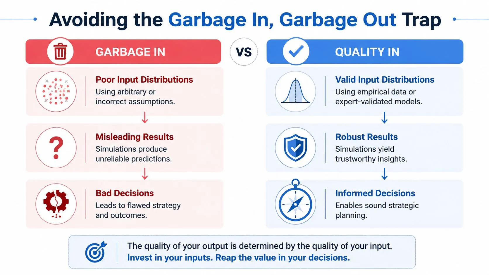
Most guides make Monte Carlo look like a mechanics problem. Pick variables, run a loop, chart the outputs. That's the easy part. The hard part is deciding what kind of randomness each input should have.
Numerous business models frequently fail in these circumstances. Research indicates that 40-60% of Monte Carlo failures in risk analysis stem from incorrect input distribution assumptions rather than algorithmic errors, according to Lumivero's discussion of Monte Carlo simulation examples.
The hardest part isn't the loop
A simulation will happily produce mathematically clean nonsense if your inputs are unrealistic.
Take startup revenue. Many teams default to a Normal distribution because it's familiar. That can be a bad choice if the variable is skewed and can't go below zero. A Normal distribution is symmetric. Revenue often isn't. It may have a long upside tail, a hard floor at zero, and occasional bursts that the bell curve treats poorly.
The danger is subtle. The output can still look impressive. You'll get percentiles, a smooth chart, and precise-looking estimates. They'll just be precise about the wrong world.
A polished percentile doesn't rescue a bad assumption. It only hides it behind cleaner math.
How to think about common distributions
You don't need to become a statistician to make better choices. You do need stronger intuition.
| Distribution | When it fits | When it misleads |
|---|---|---|
| Normal | Values cluster around a center and are roughly symmetric | Skewed business variables, hard lower bounds, heavy outliers |
| Uniform | Any value in a range is equally plausible | Cases where some outcomes are clearly more likely than others |
| Log-normal | Positive-only variables with right skew | Variables that truly center symmetrically |
| Beta | Rates and proportions bounded between zero and one | Unbounded values like revenue or cost |
A few practical examples:
- Activation rate: A bounded rate often calls for a distribution that respects lower and upper bounds.
- Revenue per account: Often better modeled with right skew than symmetry.
- Task duration: If you only know low, likely, and high, a simple bounded approximation may be more honest than pretending you know a bell curve.
Questions to ask before you choose
Before assigning any distribution, ask:
- Can this variable go negative: If not, don't use a distribution that casually generates impossible values.
- Is the data symmetric: If the downside is constrained and the upside is open-ended, symmetry is suspicious.
- Do outliers matter: Some variables are mostly calm until they aren't.
- Is the variable bounded: Rates, probabilities, and shares live inside limits.
- Do we have data or only judgment: If you're leaning on expert assumptions, be explicit about it.
Teams also improve results when they tighten the underlying data feeding those assumptions. That's why data quality work upstream of analysis often matters more than adding another chart downstream.
One more point trips people up. Distribution choice isn't only about fit. It's about decision relevance. If a small tail risk changes whether you hire, launch, or raise, you need a distribution that represents that tail credibly. Otherwise your simulation will understate the very risks leadership cares about.
Practical Implementation in Your Analytics Workflow
Theory becomes useful when you can run a model yourself, inspect it, and explain why the output deserves trust. The code isn't complicated. The discipline around it matters more.
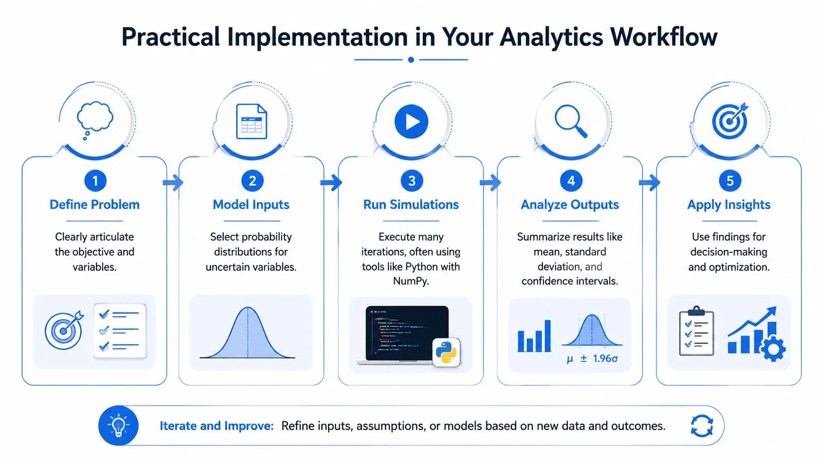
A simple Python example
Suppose you're modeling monthly profit for a new feature. You think sign-ups vary, conversion is uncertain, average revenue per converted user is skewed upward, and fixed costs are known.
import numpy as np

# Reproducibility matters
rng = np.random.default_rng(seed=42)

n_iterations = 10000

# Example inputs
signups = rng.normal(loc=5000, scale=600, size=n_iterations)
signups = np.clip(signups, 0, None)  # can't be negative

conversion_rate = rng.beta(a=8, b=32, size=n_iterations)  # bounded between 0 and 1
avg_revenue_per_user = rng.lognormal(mean=3.5, sigma=0.4, size=n_iterations)
fixed_cost = 80000

# Model
converted_users = signups * conversion_rate
revenue = converted_users * avg_revenue_per_user
profit = revenue - fixed_cost

# Summary outputs
mean_profit = profit.mean()
median_profit = np.median(profit)
p10 = np.percentile(profit, 10)
p90 = np.percentile(profit, 90)

print("Mean profit:", round(mean_profit, 2))
print("Median profit:", round(median_profit, 2))
print("10th percentile:", round(p10, 2))
print("90th percentile:", round(p90, 2))
This example does a few important things right. It sets a random seed for reproducibility. It clips impossible negative sign-ups. It uses different distributions for different kinds of variables rather than forcing everything into one pattern.
A video walkthrough can help if you want to see the mechanics visually:
How many iterations are enough
Often, many teams either stop too early or waste compute.
For high-stakes business decisions, simulations may require 50,000 to 100,000 iterations to ensure convergence, while many standard applications stabilize with 10,000. A practical test is whether key metrics change by less than 1% when you double the iteration count, as described in this practical guide to Monte Carlo convergence.
That gives you a concrete workflow:
- Start with a reasonable run size: A standard model often starts at 10,000 iterations.
- Double it and compare outputs: Check mean and important percentiles.
- Stop when decision-relevant metrics stabilize: You don't need infinite precision. You need stable enough evidence to make the call.
Decision lens: Run more iterations until the conclusion stops changing, not until the chart looks impressive.
Workflow habits that make results trustworthy
A few habits make Monte Carlo simulations much more defensible:
- Version your assumptions: Save the exact distributions and parameters used in each run.
- Separate model logic from sampling logic: Keep the business formula readable.
- Test impossible outputs: Negative users, conversion above one, and similar issues should be trapped immediately.
- Document why each distribution was chosen: Future reviewers should see the reasoning, not just the result.
This matters in team settings because someone will ask where the tails came from, why the median moved, or why this month's risk range widened. If the simulation is well structured, you can answer those questions quickly instead of reverse-engineering your own notebook.
Scaling Simulations in a Modern Data Warehouse
Monte Carlo gets more interesting when you stop treating it as a one-off notebook and start running it close to production data. That changes who can use it, how often it runs, and what decisions it can support.

Why warehouse-native simulation changes the workflow
When simulation inputs live in Snowflake, BigQuery, Redshift, or a similar platform, analysts don't need to export snapshots into disconnected spreadsheets every time they want a new run. They can pull fresh distributions from real operational data, run parameterized simulations, and publish outputs back into the same analytics environment.
That setup is especially useful for self-serve analytics. A product manager can ask for forecast ranges over current pipeline conditions. A finance lead can test planning assumptions against updated churn behavior. A data team can standardize the simulation logic once instead of rebuilding it in every ad hoc file.
Warehouse-scale execution also opens the door to parallelism. Independent simulation trials are naturally parallel-friendly, which makes the method a strong fit for modern compute systems.
Teams that want these workflows to remain manageable usually need stronger data warehouse operating practices, because simulation magnifies upstream modeling errors just as much as it magnifies uncertainty.
Precision has a compute cost
There's a tradeoff many business guides ignore. More iterations improve precision, but they also consume more compute. That matters when simulations run frequently or sit inside broader automated workflows.
Modern guides often miss the trend of using stopping rules to halt simulations early once a decision threshold is met, which is an important efficiency for teams using AI agents on warehouse data and trying to control cloud costs, as discussed in Galorath's Monte Carlo risk overview.
That idea is simple and powerful. If your decision is binary and the estimate has already stabilized enough to make the call, extra precision may not be worth paying for. In a modern analytics stack, the best simulation isn't always the longest one. It's the one that reaches sufficient confidence without waste.
This is also where architecture matters. A simulation pipeline built for repeated, parameterized runs can become part of regular planning. One built as an artisanal notebook usually can't.
Validating and Trusting Your Results
A Monte Carlo simulation isn't a crystal ball. It's a structured way to think under uncertainty. You should trust it the same way you trust any model. Conditionally, after checks.
A practical validation checklist
Before you use the output in a roadmap meeting or board deck, run through a few tests:
- Input sanity check: Are the ranges and shapes plausible given business reality?
- Boundary check: Does the model produce impossible outcomes under any sampled path?
- Sensitivity review: Which inputs drive most of the variation in the result?
- Edge-case testing: What happens under combinations that are uncomfortable but still plausible?
- Decision stability: If assumptions move a little, does the recommendation flip?
A useful habit is to show both the result and the assumption sheet together. That forces the conversation onto model quality instead of false certainty.
Trust the simulation when it clarifies uncertainty. Distrust it when it pretends uncertainty has disappeared.
The best Monte Carlo work doesn't just produce a prettier forecast. It sharpens judgment. It tells you where the model is fragile, which assumptions deserve scrutiny, and whether the decision still looks good when reality refuses to behave like an average month.
If your team wants to run this kind of analysis without turning data analysts into a ticket queue, Querio helps teams work directly on warehouse data with AI coding agents and Python-first workflows. That makes it easier to build, repeat, and operationalize simulations and other advanced analytics without waiting on a traditional BI backlog.