Data Warehouse Query Explained for Modern Data Teams

A product dashboard is spinning while a board meeting waits for the answer. The SQL may look short, but the warehouse still has to find the relevant data, decide how to move it, coordinate compute, and return the result while other users compete for the same resources. By the time the chart appears, the problem may be storage layout, an inefficient join, a changed execution plan, or simple workload contention.

A data warehouse query is more than SQL text. It's a measurable event with a start time, duration, row count, execution plan, concurrency context, and usage pattern. Once you see the query that way, performance troubleshooting becomes less about memorizing syntax tips and more about following the request through the warehouse layer by layer.

Table of Contents

• What a Data Warehouse Query Really Is
• How a Query Executes Inside a Modern Warehouse
  • Parse the request
  • Build a logical plan
  • Optimize the route
  • Execute in parallel
• Why Partitioning and Storage Layout Decide Query Speed
  • Diagnose the physical layer first
• Writing Efficient Queries That Scale
  • Filter before expensive operations
  • Project only the columns you need
  • Pre-aggregate recurring metrics
  • Keep join keys usable
  • Stage very large transformations
• From Analyst Bottleneck to Self-Serve Query Workflows
  • Give different users different interfaces
  • Optimize the workload, not just the statement
• Monitoring and Troubleshooting Query Performance
  • Start with the recurring request
  • Trace the regression
• Key Takeaways for Data Teams

What a Data Warehouse Query Really Is

A product leader asks why a weekly activation report takes seconds in a notebook but minutes in the company dashboard. The SQL may be identical. The warehouse still has to interpret the request, locate the relevant data, combine records, allocate compute, and return the result alongside other work.

A data warehouse query is a request to retrieve, combine, summarize, or transform data for analysis. A product manager may ask for weekly activation by acquisition channel. A finance leader may need revenue grouped by region and customer segment. A data scientist may join event data with account attributes before building a model.

That work differs from an operational lookup. An application database might find one customer by an identifier. An analytical query can read broad sections of several tables, join datasets, filter rows, and calculate aggregates before returning a small result.

A library provides a useful comparison. An operational lookup asks for one specific book. An analytical query asks a librarian to examine an archive, compare records across collections, and prepare a summary. The answer may fit on one page, while producing it requires much more work behind the scenes.

Practical rule: Judge a warehouse query by the work required to produce its result, not by the length of its SQL.

Warehouses are built for reporting, exploration, recurring dashboards, forecasting, and other workloads that analyze data at scale. Several users may run similar requests simultaneously. A dashboard can also repeat the same query whenever someone opens it, turning a modest request into a recurring load.

Query analysis therefore needs more than a text search for a slow statement. Treat each request as an operational event with a start time, duration, execution plan, row count, concurrency context, and usage pattern. Microsoft Fabric, for example, documents query insight views for execution history, long-running queries, and frequently run queries, including fields such as elapsed time, row count, run count, and median runtime in its monitoring model Microsoft's query insight documentation.

A query may slow down because it reads too much data, waits behind other work, receives an inefficient execution plan, or repeats expensive processing. The SQL is the instruction. The warehouse is the system that interprets and carries it out.

For a broader foundation, this explanation of query language separates the language used to express a request from the system that executes it. That distinction helps analysts connect a wording change in SQL to the operational reason it improves performance.

How a Query Executes Inside a Modern Warehouse

Take a recurring dashboard request:

SELECT
  customer_segment,
  SUM(revenue) AS total_revenue
FROM orders
WHERE order_date >= DATE '2026-01-01'
GROUP BY customer_segment;

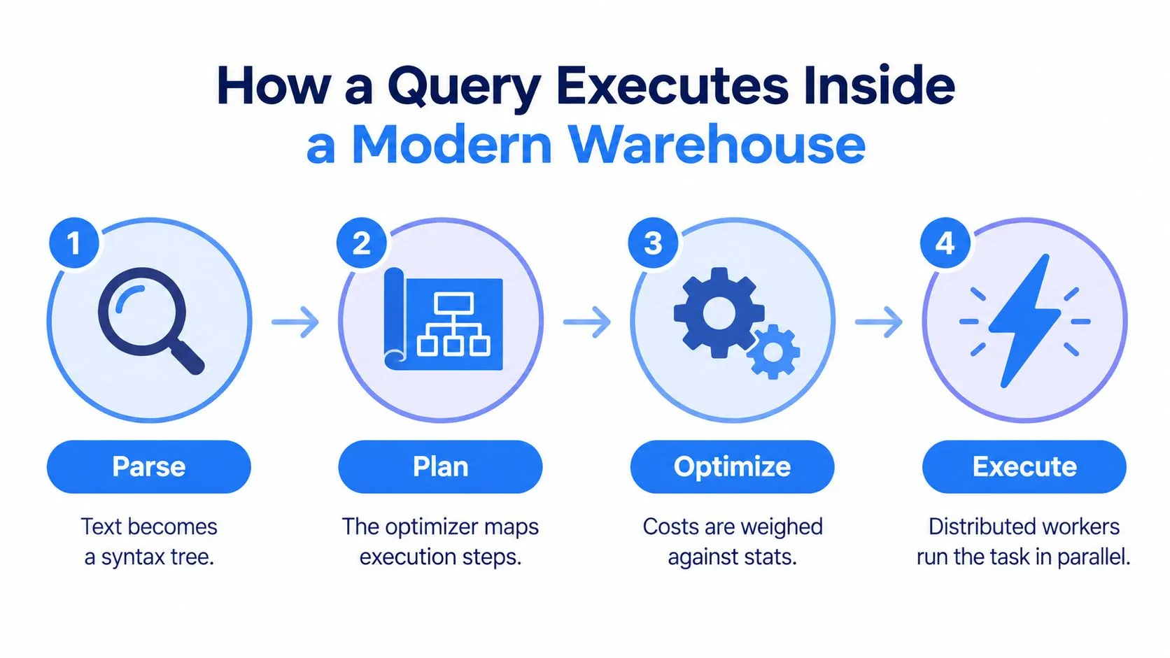
The request looks simple. Inside the warehouse, it passes through several distinct stages before the dashboard receives a result.

Parse the request

First, the warehouse parses the SQL. It checks whether the statement follows the expected grammar, resolves table and column names, and turns the text into an internal representation, often described as a syntax tree.

At this point, the system isn't deciding whether the query is efficient. It's determining what the request means. If a column is misspelled or a table is unavailable, the query can fail before execution begins.

Build a logical plan

Next, the warehouse converts the request into logical operations. In this example, the operations include reading orders, applying a date filter, grouping rows by customer segment, and calculating a sum.

The logical plan describes the required result without yet committing to a physical route. It's similar to telling a warehouse foreman, “Find qualifying boxes, group them by category, and count their contents,” without specifying which aisles workers should use.

Optimize the route

The optimizer chooses a physical execution plan. It may decide which table to read first, where to apply filters, how to perform joins, whether to use a materialized view, and how to distribute work across compute resources.

Think of the optimizer as a logistics planner. It compares possible routes based on available information about table size, data distribution, storage layout, and expected work. Two warehouses can receive identical SQL and choose different plans because their storage engines, statistics, clustering, indexes, compute settings, and optimizer logic differ.

The system's goal isn't to make the SQL look elegant. It's to reduce the work needed to produce the correct result.

Execute in parallel

Finally, workers execute the physical plan. A large scan can be divided into work units, with multiple workers reading different portions of storage at the same time. Those workers filter rows, calculate partial aggregates, exchange intermediate results, and combine them into the final answer.

Columnar storage can reduce unnecessary reading when the query needs only a small set of columns. In the example, the warehouse needs the date, segment, and revenue fields, not every attribute stored in the orders table. The benefit depends on the platform and physical layout, but the principle is consistent: less data read usually means less work to process.

A query may also spend time waiting. Workers can queue behind other requests, wait for memory, or exchange data across nodes. That's why execution time isn't determined only by the SQL operations. It reflects the plan, the data, the available resources, and the workload running at the same time.

The practical meaning of query execution time is therefore broader than the time spent “running the statement.” It's the elapsed experience of a request moving through parsing, planning, scheduling, processing, and result delivery.

The warehouse exposes some of these stages through an execution plan and runtime profile. Those tools let you ask a more useful question than “Why is this query slow?” You can ask, “Which stage is doing more work than expected?”

The video below provides another visual introduction to the execution path.

Why Partitioning and Storage Layout Decide Query Speed

A well-written query can still perform poorly if the warehouse has to inspect far more data than the question requires. The physical storage layer determines how selectively the engine can read data.

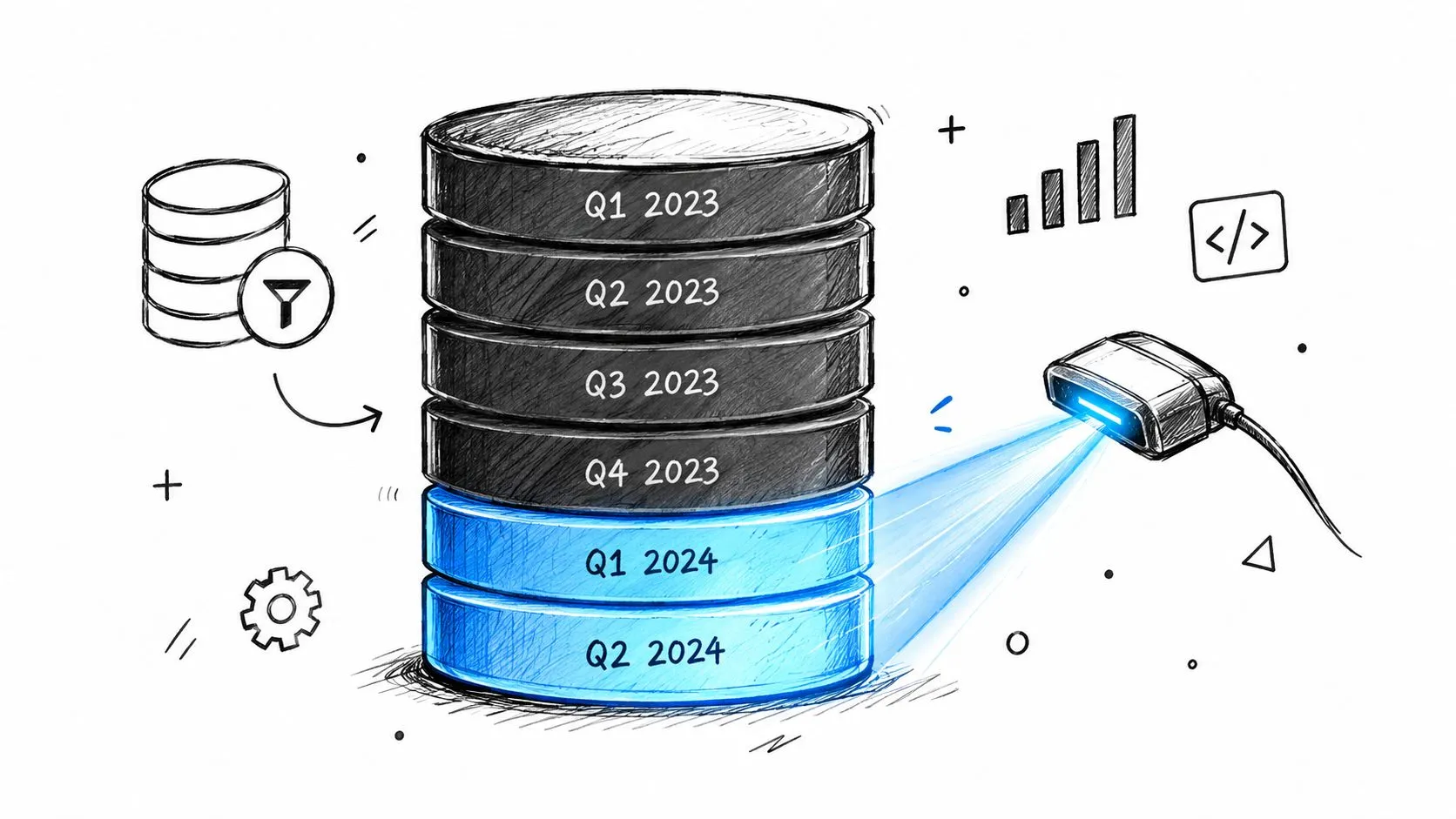
Partitioning divides a table into logical sections, often by a field such as date. Suppose a sales table is partitioned by order month. A report for one month can target the relevant partition instead of scanning the complete table. The SQL may not change, but the amount of data considered by the engine can change substantially.

Clustering organizes related values so the warehouse can narrow its scan more effectively. If users regularly filter by region or account identifier, a suitable layout can make those filters more useful. The exact implementation differs across platforms, so teams should inspect the platform's execution profile rather than assume that a declared layout automatically improves every query.

Materialized views store the result of an expensive transformation so recurring requests can read prepared data instead of rebuilding the same joins and aggregations. They're useful when the underlying data and metric definition support refreshes that meet the business need.

Indexes, where supported and appropriate, provide another access path for locating relevant records. They can help selective lookups, although their value depends on the warehouse engine, table design, write patterns, and query shape.

Research on distributed data warehouse processing identifies partitioning, indexing, materialized views, and parallel execution as key ways to reduce runtime work. The cited research reports that these techniques can cut execution time by up to 45% and improve resource utilization by about 30% in cloud data warehouse workloads distributed data warehouse query processing research.

Those figures are not a promise for every schema. They show why storage design deserves attention before a team rewrites a complicated query. If the engine reads irrelevant partitions, repeatedly computes the same summary, or moves too much data between workers, syntax changes alone may have limited impact.

Diagnose the physical layer first

Start with the execution plan and ask:

• Did the filter eliminate partitions, or did the engine scan broadly?
• Which operator read the most data?
• Did a join cause a large redistribution between workers?
• Did the query use a materialized view or summary structure where one exists?
• Are estimated row counts close to actual row counts?

A date filter can fail to prune partitions if it wraps the partition key in a function or applies a transformation the engine can't use for elimination. A join can become expensive when one side is much larger than expected or when the join keys distribute data unevenly.

Teams working with distributed systems can also review how hash partitioning improves load balancing. The central idea is simple: query speed depends partly on whether the warehouse can divide work evenly. One overloaded worker can hold up the result while others sit idle.

Writing Efficient Queries That Scale

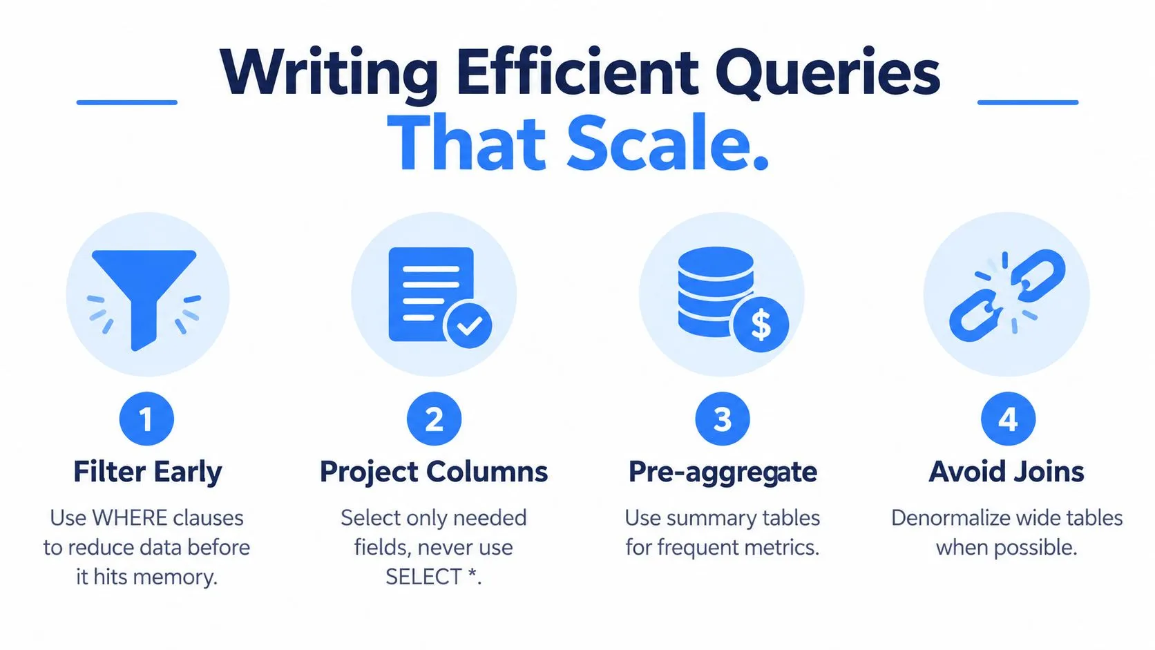
Query writing still matters, especially when the warehouse must process large tables under concurrent analytical workloads. The strongest habits reduce data early, avoid unnecessary movement, and prevent repeated work.

Filter before expensive operations

Apply selective filters as close to the source table as the query semantics allow. Filtering after a broad join can force the warehouse to combine rows that the final answer would discard.

Less selective shape:

SELECT
  c.segment,
  SUM(o.revenue)
FROM orders o
JOIN customers c ON o.customer_id = c.customer_id
GROUP BY c.segment;

More selective shape:

SELECT
  c.segment,
  SUM(o.revenue)
FROM orders o
JOIN customers c ON o.customer_id = c.customer_id
WHERE o.order_date >= DATE '2026-01-01'
GROUP BY c.segment;

The second version gives the optimizer an earlier opportunity to reduce the order rows entering the join. Whether the engine pushes the predicate automatically depends on its optimizer and the query structure, so inspect the plan.

Project only the columns you need

SELECT * asks the warehouse to retrieve every selected column, even when the dashboard uses only a few. It also makes downstream models fragile because a schema change can increase the work without changing the visible query.

Prefer:

SELECT customer_id, order_date, revenue
FROM orders;

over:

SELECT *
FROM orders;

Columnar systems can benefit when a query references fewer columns, because the engine has less data to read and transfer. Explicit projection also documents the fields that the analysis depends on.

Pre-aggregate recurring metrics

If a dashboard repeatedly calculates the same daily revenue summary, consider maintaining a governed summary table or materialized view. The dashboard can then read the prepared grain instead of joining and aggregating raw events every time.

This approach requires ownership. Teams need to define refresh behavior, metric logic, late-arriving data handling, and permissions. A summary table that nobody trusts only moves the problem elsewhere.

Keep join keys usable

Functions and implicit type conversions on join keys can make optimization harder. Instead of transforming both sides inside the join, normalize the relevant values upstream when possible.

Less direct:

ON LOWER(a.email) = LOWER(b.email)

More operationally predictable:

ON a.normalized_email = b.normalized_email

The second design shifts normalization into a controlled data transformation. It can also make data quality checks easier because the team can test the normalized field before users depend on it.

Stage very large transformations

A single statement may be convenient during exploration, but enormous transformations can become difficult to explain and troubleshoot. Breaking work into staged, well-named models can expose intermediate row counts, simplify retries, and make performance regressions easier to isolate.

Independent warehouse benchmarking commonly uses TPC-H and TPC-DS-style workloads because business-oriented decision-support queries stress joins, aggregations, and concurrency. The cloud data warehouse benchmark description describes TPC-H as a suite of business-oriented ad hoc queries and concurrent data modifications. That focus mirrors the conditions that expose weak query design.

Query Habit	Typical Impact	When It Matters Most
Filter early	Reduces rows entering joins and aggregations	Large fact tables and date-bounded reports
Project required columns	Reduces unnecessary reads and transfers	Wide tables and dashboard queries
Pre-aggregate recurring metrics	Avoids repeated transformation work	Frequently refreshed reports
Keep join keys usable	Gives the optimizer a clearer path	Large joins and shared dimensional keys
Stage complex transformations	Makes work easier to inspect and retry	Long pipelines and changing business logic

Use query optimization techniques as a practical reference, but don't apply rules mechanically. The execution plan remains the authority. A rewrite that looks cleaner may not change the physical work, while a small change to a filter, key, or aggregation boundary can have a substantial effect.

From Analyst Bottleneck to Self-Serve Query Workflows

Many data teams become a human API. A product manager asks for activation by cohort, a founder requests a revenue cut, and an engineer needs a customer list for an investigation. Each request may be reasonable, but the queue grows faster than the team can answer it.

The warehouse already contains the information. The bottleneck is often the path between a business question and a trustworthy query. That path includes schema knowledge, metric definitions, permissions, SQL generation, validation, and interpretation.

Self-serve workflows change the role of the data team. Instead of manually answering every request, data engineers can maintain the structures that let others answer routine questions safely. Those structures include documented models, governed metrics, reusable notebooks, access controls, validation checks, and monitoring.

Give different users different interfaces

A data engineer may prefer a SQL editor and execution plan. An analyst may work best in a notebook that combines Python, SQL, charts, and written reasoning. A product leader may ask a natural-language question and review the generated SQL before using the result.

Custom Python notebooks are useful when the analysis needs repeatable logic, exploratory code, or a record of how an answer was produced. AI coding agents can help draft queries and transformations, but they still need warehouse permissions, schema context, tests, and human review. Natural language can reduce the cost of asking a question, but it doesn't remove the need to define the metric correctly.

Governance should sit inside the workflow rather than appear as a final approval step. A self-serve user should know which tables are trusted, which fields contain sensitive information, and which definitions the company uses for terms such as active customer or retained account.

Optimize the workload, not just the statement

The operational challenge is shifting from writing SQL to controlling cost and latency under mixed workloads. A warehouse may serve scheduled transformations, interactive dashboards, exploratory notebooks, application requests, and automated agents at the same time.

Recent trend coverage reports that Snowflake's Query Acceleration Service was handling over 30% of queries by mid-2025, with an average 40% performance improvement, and describes automatic query rewriting, workload management, and serverless scaling as part of the industry's response data warehousing trends coverage. Those are reported platform and trend claims, not a universal result for every warehouse or query.

The management question is therefore broader than “Can this query run?” Ask whether it should run interactively, whether it can use a prepared result, whether it belongs in a separate workload, and whether the user needs raw rows or a governed answer.

A mature data team creates those paths. It provides safe access to live data, makes common metrics reusable, and monitors the queries that consume shared capacity. Analysts spend more time on ambiguous business questions, while product teams handle routine exploration without opening a ticket for every slice of data.

Monitoring and Troubleshooting Query Performance

A dashboard that usually responds in seconds begins timing out after a schema change. The SQL text appears unchanged, so the first task is not rewriting the statement. It is finding evidence of what changed inside the warehouse.

Query history, execution plans, and runtime statistics provide that evidence. Together, they let a team compare the same data warehouse query across executions and separate a parsing or plan change from a storage, workload, or concurrency problem.

Microsoft announced general availability of Query Store for Azure SQL Data Warehouse on January 31, 2019. The announcement describes automatic capture of query history, plans, and runtime statistics, with data separated into time windows for examining usage patterns and plan changes. Amazon Redshift documentation describes a guaranteed seven-day query history, while Snowflake's QUERY_HISTORY view supports analysis over the last 365 days the Query Store announcement and warehouse history details.

Start with the recurring request

Identify the exact query or query pattern, then compare recent executions with earlier ones. The comparison should answer five practical questions:

• Elapsed time: Did execution itself become slower, or did the request spend longer waiting in a queue?
• Row count: Did the query start processing or returning more rows?
• Run frequency: Is a dashboard, notebook, or service sending the request more often?
• Median runtime: Is the slowdown consistent across executions, or does one run reflect an unusual condition?
• Plan shape: Did the warehouse stop pruning partitions, choose another join strategy, or add an expensive sort?

Microsoft Fabric documents views such as exec_requests_history, long_running_queries, and frequently_run_queries. Their fields include total_elapsed_time_ms, row_count, number_of_runs, and median_total_elapsed_time_ms. Databricks SQL warehouse monitoring similarly surfaces running and queued queries, plus history fields such as start time, duration, fetch time, and query source documented warehouse query monitoring concepts.

Trace the regression

Suppose the newer execution scans more of the orders structure after the schema change. Query history shows unchanged SQL, while the newer plan reads additional data. The execution profile then reveals that the date predicate no longer removes the expected storage sections.

That sequence narrows the investigation. Check whether the partition key changed, whether a cast or function now surrounds the filter, whether statistics are stale, or whether the dashboard references a view whose definition has changed. Each possibility affects a different layer of the query path, so the plan and runtime profile prevent guesswork.

An unchanged plan with higher elapsed time points toward concurrency or queue behavior. The query may be waiting behind another workload rather than performing more internal work. Higher row counts suggest changed upstream volume or filter semantics. Sharp runtime variation calls for a comparison of resource availability and execution conditions across runs.

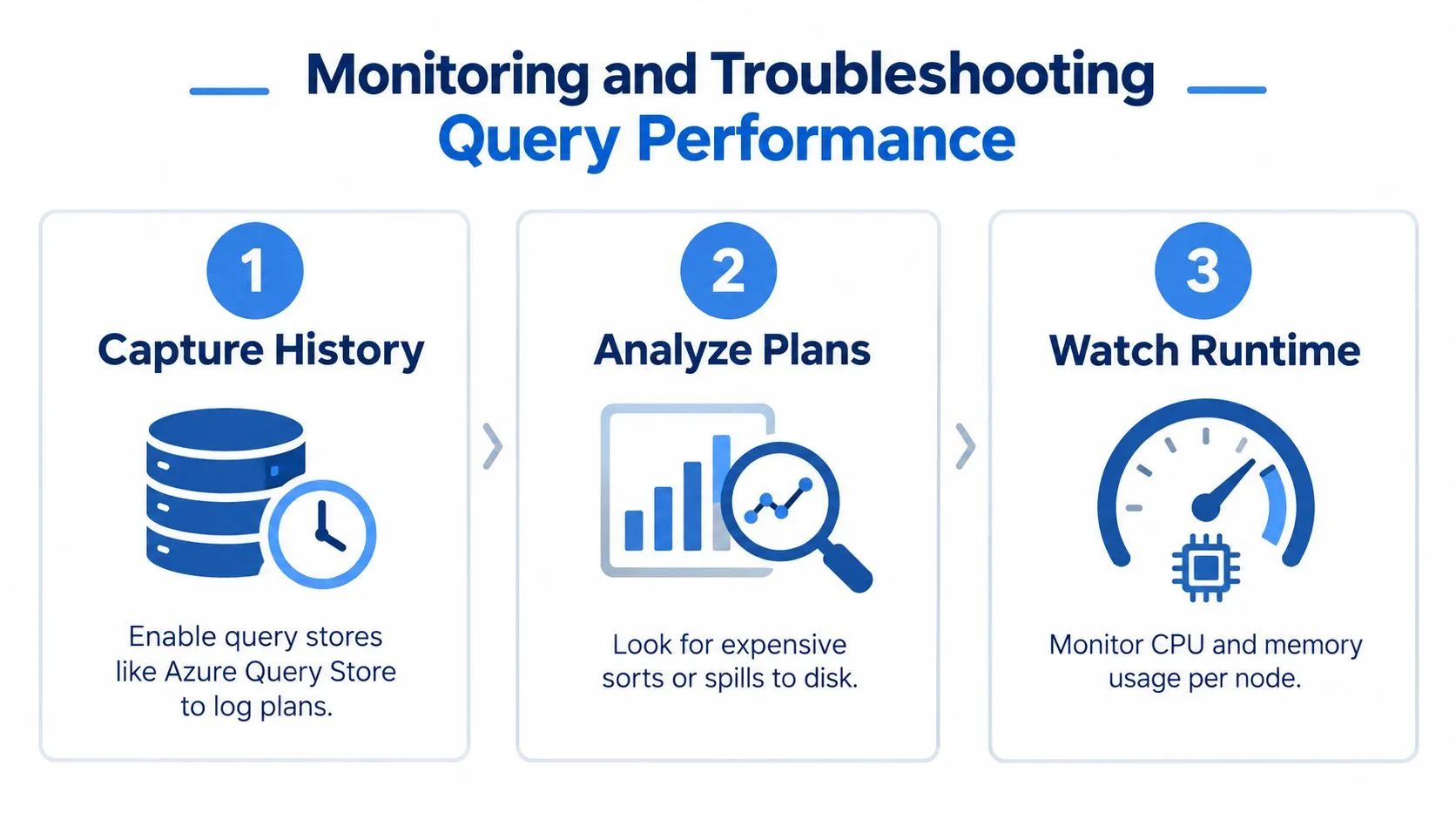
Evidence beats intuition: A slow query is a symptom. History and plans show whether the cause is more data, a different execution route, resource contention, or repeated execution.

Prioritize queries that are both expensive and frequent. One long-running investigation may deserve attention, yet a modest query repeated by every dashboard viewer can consume more shared capacity over time. Monitoring turns that distinction into a measurable decision.

Key Takeaways for Data Teams

A data warehouse query is a request moving through a system, not just a string of SQL. Its performance reflects parsing, planning, physical execution, storage layout, concurrency, and result delivery.

Keep four ideas in view:

• Measure the event: Track elapsed time, row counts, run frequency, queue behavior, and execution plans.
• Reduce the work: Partitioning, clustering, materialized views, usable join keys, and selective projections help the warehouse avoid unnecessary processing.
• Write for scale: Filter early, select required columns, pre-aggregate recurring metrics, and stage transformations that are difficult to inspect as one statement.
• Operate with evidence: Use query history and runtime profiles to compare regressions, identify long-running statements, and prioritize frequently executed workloads.

Modern observability makes those practices concrete. Fabric's documented views distinguish execution history, long-running queries, and frequently run queries, while Databricks exposes running, queued, and historical request details. These metrics help data teams move from “the dashboard feels slow” to a specific diagnosis.

The strategic payoff is larger than faster reports. When teams understand execution and build governed self-serve workflows, data engineers stop acting as ticket-takers and start maintaining analytics infrastructure that can support the business as usage expands.

---

Querio connects AI coding agents and custom Python notebooks directly to warehouse data, helping technical and non-technical users turn questions into SQL-backed analysis without waiting for an analyst to answer every request. Visit Querio to explore a self-serve workflow for querying and analyzing your warehouse.