Master Inner Join Outer Join SQL: 2026 Practical Guide

You're probably looking at two dashboards that should agree and don't. Sign-ups say one thing. Activation says another. Finance has a third number pulled from the warehouse, and nobody's sure whether the problem is user behavior, broken tracking, or the SQL.

That's where inner join outer join sql stops being a syntax lesson and becomes an analytics skill. Joins decide which rows survive your query. They also decide whether your report tells the clean story of matched records only, or the messier but often more useful story of what's missing.

Initially, developers learn INNER JOIN because it feels safe. Later, they discover that LEFT, RIGHT, and FULL OUTER JOIN are often what expose onboarding gaps, data integrity issues, and silent reporting errors. The trade-off is that the more complete query is often slower, noisier, and easier to misread if you don't handle NULLs carefully.

Here's the quick version before we go deeper.

Table of Contents

• The Analytics Puzzle Missing Data and Mismatched Numbers

• The Foundation INNER JOIN for Core Intersections

  • What INNER JOIN actually returns

  • Why teams default to INNER JOIN

• Expanding Your View with OUTER JOINs

  • LEFT JOIN for finding drop-offs

  • RIGHT JOIN for integrity checks

  • FULL OUTER JOIN for reconciliation

  • What each outer join is really doing

• Visualizing the Difference A Side-by-Side Comparison

  • INNER vs OUTER JOIN At a Glance

• Handling NULLs and Duplicates The Hidden Reporting Traps

  • Why NULLs break business metrics

  • Safer patterns for self-serve reports

• Performance Optimization for Data Warehouses

  • Why INNER JOIN usually runs faster

  • A faster anti-join pattern

• Choosing the Right Join for Your Analytics Workflow

  • A practical decision rule

The Analytics Puzzle Missing Data and Mismatched Numbers

A product manager pulls two lists. One comes from users, filtered to everyone who signed up this week. The other comes from events, filtered to everyone who completed a key action. The counts don't line up.

That mismatch leads to the usual questions. Did users fail to activate. Did tracking drop events. Did a warehouse sync lag. Or did the SQL exclude users because the query only kept records that matched across both tables?

Joins exist because business data rarely lives in one place. User profiles sit in one table, event logs in another, subscriptions in a third, and CRM records somewhere else entirely. If you don't choose the join deliberately, your report can look precise while hiding the rows that matter most.

A simple example makes the risk obvious:

• INNER JOIN query: shows only users who both signed up and generated an event

• LEFT JOIN query: shows all signed-up users, including those with no event

• FULL OUTER JOIN query: shows all users and all events, even when one side doesn't have a partner row

The question isn't just “How do I combine these tables?” It's “Which missing records am I willing to hide?”

That's why join strategy sits so close to data quality. Before people argue about conversion, retention, or churn, they need to trust that the report includes the right population. If your team is already dealing with inconsistent inputs, it helps to tighten the foundation first with stronger data quality practices for analytics.

The practical takeaway is simple. If the business question is about confirmed relationships, use an intersection. If the business question is about gaps, drop-offs, exceptions, or reconciliation, matched rows alone won't be enough.

The Foundation INNER JOIN for Core Intersections

An INNER JOIN returns only rows where the join condition matches on both sides. In plain English, it keeps the overlap.

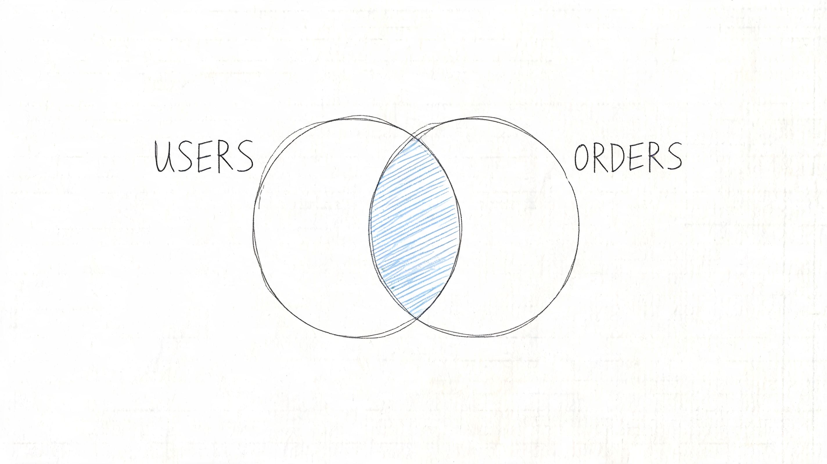
If users.user_id = orders.user_id, then you get customers who placed orders. If a user never ordered, that user disappears. If an order points to a missing user record, that order disappears too.

What INNER JOIN actually returns

Start with two simple tables:

users

orders

Query:

SELECT
  u.user_id,
  u.name,
  o.order_id
FROM users u
INNER JOIN orders o
  ON u.user_id = o.user_id;

Result:

Ben is gone because there's no matching order. That's exactly what you want for questions like:

• Revenue analysis: customers linked to purchases

• Feature adoption: accounts linked to product usage

• Support reporting: tickets linked to known customers

The join type is old, standard, and still dominant. The INNER JOIN was first formally introduced in the SQL-86 standard, and a 2024 analysis of 1.2 billion anonymized BigQuery queries found that INNER JOIN made up 72% of all join operations.

Why teams default to INNER JOIN

INNER JOIN is the workhorse because most core reporting starts with relationships the business already trusts. Paid subscription tied to customer. Event tied to session. Opportunity tied to account.

It also aligns with how people think. They want the valid overlap, not the messy fringe around it.

A quick walkthrough helps if you want to see the syntax in action:

Practical rule: Use INNER JOIN when missing relationships should be excluded by design, not investigated.

There's one more reason analysts reach for it first. It often keeps reports cleaner and query plans simpler. That doesn't mean it's always correct. It means it's the best starting point when the business metric is defined by confirmed matches.

If you want more examples built around common warehouse patterns, this guide on inner join SQL usage in analytics is a useful companion.

Expanding Your View with OUTER JOINs

INNER JOIN tells you what matched. OUTER JOINs tell you what didn't, and that's often where product and operations teams find the true story.

When a stakeholder asks, “Which users signed up but never activated?” they're not asking for overlap. They're asking for the missing side of the relationship. That's outer join territory.

LEFT JOIN for finding drop-offs

A LEFT JOIN keeps every row from the left table and adds matching rows from the right table. If there's no match, the right-side columns become NULL.

Using the same example:

SELECT
  u.user_id,
  u.name,
  o.order_id
FROM users u
LEFT JOIN orders o
  ON u.user_id = o.user_id;

If Ben has no orders, he still appears. His order_id is NULL.

That makes LEFT JOIN the most common outer join for analytics questions like:

• Activation gaps: users with no onboarding event

• Sales coverage: leads with no follow-up task

• Subscription risk: customers with no recent usage

A simple filter turns the joined result into a gap finder:

SELECT
  u.user_id,
  u.name
FROM users u
LEFT JOIN orders o
  ON u.user_id = o.user_id
WHERE o.order_id IS NULL;

That query doesn't show purchasers. It shows everyone who never purchased.

RIGHT JOIN for integrity checks

A RIGHT JOIN is the mirror image. It keeps every row from the right table and matches from the left.

SELECT
  u.user_id,
  u.name,
  o.order_id
FROM users u
RIGHT JOIN orders o
  ON u.user_id = o.user_id;

In business analytics, RIGHT JOIN is less common because many practitioners read queries left to right and prefer to put the primary population first. Still, it's useful when the right-side table is the thing you must preserve.

For example, if you want every order whether or not a valid user record exists, a right join exposes orphaned transactions. That's a data integrity problem, not just a reporting quirk.

FULL OUTER JOIN for reconciliation

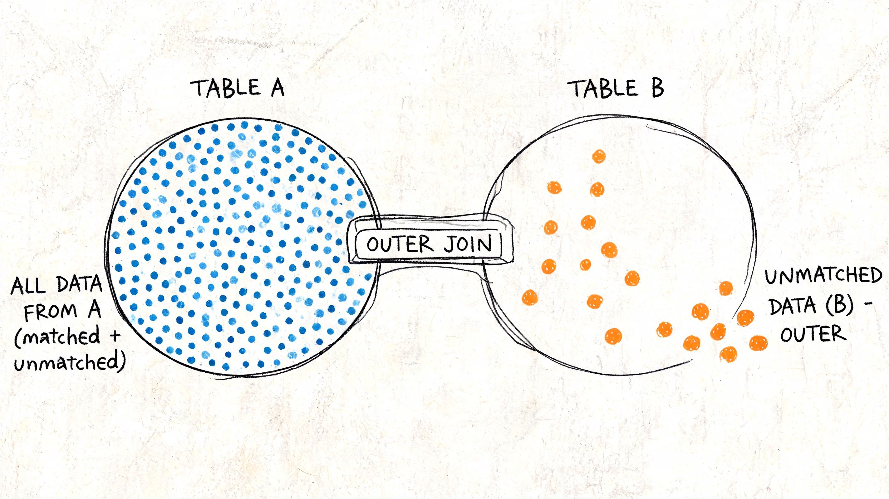
A FULL OUTER JOIN keeps all rows from both tables. Matched rows merge. Unmatched rows on either side remain, with NULLs filling the missing side.

SELECT
  u.user_id,
  u.name,
  o.order_id
FROM users u
FULL OUTER JOIN orders o
  ON u.user_id = o.user_id;

This is the join you use when reconciling systems. Warehouse table against finance export. CRM account list against billing records. Legacy product IDs against a new dimension table.

It's rarely the first join to reach for in a dashboard, but it's the right one when completeness matters more than neatness.

Outer joins are how analysts answer “Who is missing?” instead of only “Who matched?”

That's not a small distinction. A 2023 StrataScratch benchmark on employee-bonus data found that OUTER JOINs exposed 27 missing bonus records out of 30 employees, a 90% completeness gap that an INNER JOIN missed entirely.

What each outer join is really doing

Here's the business framing:

• LEFT JOIN: preserve your primary population, then inspect who failed to connect to downstream activity

• RIGHT JOIN: preserve the dependent dataset, often to catch broken references

• FULL OUTER JOIN: preserve both sides for audits, migration checks, and reconciliation work

The trap is using an outer join just because it feels safer. If your metric is “paid customers with successful charges,” a left or full join can add noise and duplicate null-heavy rows you never intended to analyze.

Use outer joins when missing records are part of the question. If they aren't, they're often the wrong tool.

Visualizing the Difference A Side-by-Side Comparison

When people struggle with inner join outer join sql, the confusion usually isn't syntax. It's mental model. Which rows survive. Which disappear. Which come back as NULL.

This visual works well as a cheat sheet when you're moving quickly between reporting tasks.

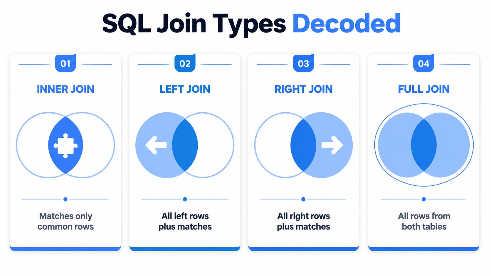
INNER vs OUTER JOIN At a Glance

A useful shortcut:

• If the left table is your business population, start with LEFT JOIN

• If you only care about confirmed relationships, choose INNER JOIN

• If you're checking whether either system is missing records, reach for FULL OUTER JOIN

Most dashboard queries need fewer rows, not more. Most audit queries need more rows, not fewer.

That distinction clears up a lot of join decisions. Product metrics tend to begin with a population definition. Reconciliation work begins with distrust. Your join should reflect that.

There's also a communication advantage. A PM usually understands “show me all sign-ups, even those with no activity” faster than they understand “left-preserving outer join semantics.” Framing the question first often gets you to the right query faster than debating syntax.

Handling NULLs and Duplicates The Hidden Reporting Traps

A PM opens a dashboard and sees active users drop after a new table gets joined in. No product change caused it. The query did.

OUTER JOIN problems usually show up after the join, in aggregation, filtering, and labeling. That is why teams can approve a query in SQL review and still ship a misleading report in Looker, Hex, or a self-serve layer. The join ran as written. The metric logic did not survive the new row shape.

Why NULLs break business metrics

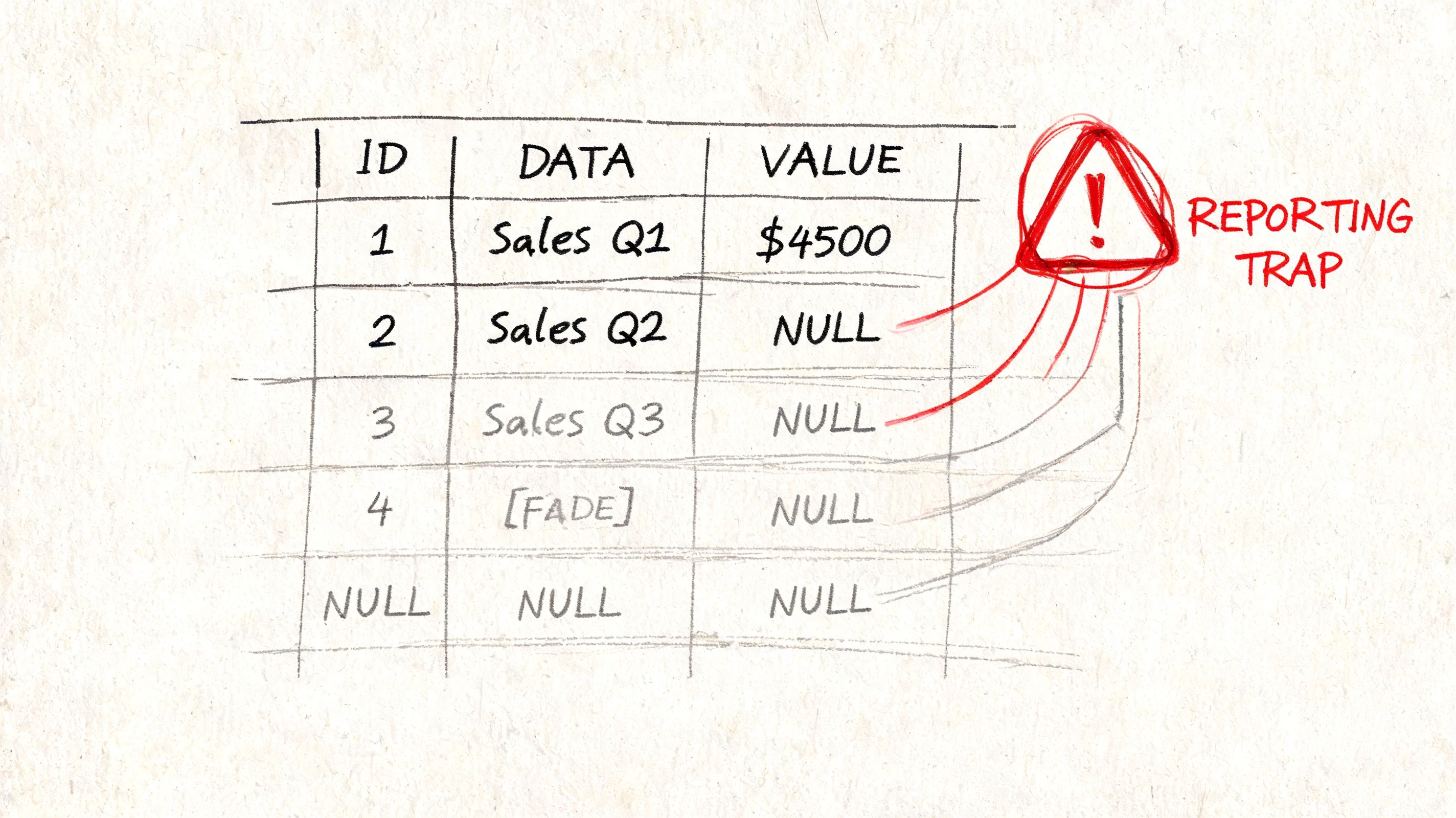
Suppose you join users to orders with a left join. Every user stays in the result. Users without orders get NULL in the order fields.

That sounds harmless until someone aggregates:

SELECT
  COUNT(*) AS joined_rows,
  COUNT(o.order_id) AS matched_orders
FROM users u
LEFT JOIN orders o
  ON u.user_id = o.user_id;

COUNT(*) returns all joined rows. COUNT(o.order_id) ignores null order IDs. Both are valid, but they answer different business questions.

In reporting, that distinction matters fast. A PM reading COUNT(o.order_id) as "users in the dataset" gets an undercount. An analyst filtering WHERE o.status != 'cancelled' can also turn a left join into an inner join by accident, because rows with NULL status disappear.

Then duplication enters the picture.

If one user has five orders, that user appears five times after the join. Any downstream metric that assumes one row per user is now wrong unless the query restores the user-level grain with COUNT(DISTINCT u.user_id) or pre-aggregates orders first.

A join changes row grain. Reports break when the metric still assumes the old grain.

That pattern shows up constantly in self-serve BI. Business users usually inspect the columns they added. They inspect row multiplication less often. Modern analytics tools need to make that grain shift obvious, or analysts end up cleaning the same mistakes from ad hoc dashboards every week.

Safer patterns for self-serve reports

The practical fix is to decide the reporting grain before writing the aggregate. If the output should be one row per user, shape the orders table to one row per user first, then join.

• Replace display nulls deliberately: use COALESCE or ISNULL when blanks would confuse report readers

• Aggregate before joining: summarize child tables to the business grain you need

• Count with intent: choose COUNT(*), COUNT(column), or COUNT(DISTINCT ...) based on the metric definition

• Watch post-join filters: conditions on right-table columns can remove unmatched rows

Examples:

SELECT
  u.user_id,
  COALESCE(SUM(o.amount), 0) AS revenue
FROM users u
LEFT JOIN orders o
  ON u.user_id = o.user_id
GROUP BY u.user_id;

And for cleaner labels:

SELECT
  u.user_id,
  COALESCE(o.status, 'No order') AS order_status
FROM users u
LEFT JOIN orders o
  ON u.user_id = o.user_id;

For teams building reusable metrics, standard null handling helps prevent each analyst from inventing a different fallback rule. A good reference is SQL IF NULL handling patterns, especially when blanks, zeros, and "no matching record" mean different things in downstream dashboards.

A short review catches most of these traps:

1. Check the grain first: define what one row represents after the join

2. Test unmatched records: filter WHERE right_table.key IS NULL and confirm that those rows make business sense

3. Separate missing from zero: NULL, 0, and 'No order' communicate different states

4. Pre-aggregate child tables: if the report is user-level, make the joined table user-level too

Tools like Querio help by pushing these choices closer to the metric layer instead of leaving them buried in one analyst's custom SQL. That matters in self-serve analytics, where the biggest reporting failures rarely come from syntax mistakes. They come from joins that changed the meaning of the result set without anyone noticing.

Performance Optimization for Data Warehouses

A join that looks harmless in a BI tool can become the slowest step in your warehouse once it feeds a dashboard, a scheduled model, and three ad hoc follow-up cuts. Join choice affects accuracy, but it also changes scan volume, memory use, shuffle cost, and how quickly a self-serve query returns before a PM gives up and exports to CSV.

INNER JOIN is usually cheaper because the engine can work with the overlap between two tables and drop irrelevant rows earlier. LEFT, RIGHT, and FULL OUTER JOIN preserve more of the Venn diagram, which is often correct for the business question, but more expensive for the warehouse.

Why INNER JOIN usually runs faster

In practice, the cost difference shows up in intermediate results. If a query keeps unmatched rows alive for several more steps, the warehouse still has to scan them, sort them, shuffle them across nodes, and hold them in memory long enough to finish the plan. Analysts usually notice this as a query that suddenly feels heavy after one join change.

A Ben Nadel benchmark on outer-join versus inner-join patterns points in the same direction. The broader lesson is simple. If the report does not need unmatched rows, preserving them adds cost without adding insight.

That trade-off matters even more in modern analytics workflows. A slow join is rarely isolated to one analyst's notebook. It often sits inside a semantic layer, powers a shared metric, or gets reused by self-serve BI users who have no reason to inspect the generated SQL.

A few habits usually pay off:

• Cluster, partition, or index join keys where the platform allows it: customer_id, account_id, order_id

• Filter inputs before joining: reduce each side at the cheapest stage

• Select only the columns you need: wide intermediate tables slow everything down

• Pre-aggregate before the join when the report grain is higher than the event grain: join daily user metrics to users, not raw clickstream to users

• Use FULL OUTER JOIN sparingly: it is useful for reconciliation, but expensive for everyday reporting

There is a modeling choice here too. One oversized query that tries to answer every future question usually performs worse than a sequence of smaller, well-defined steps. Warehouses optimize clearer plans more reliably, and other analysts can audit them faster.

For teams tuning recurring reports, this guide on optimizing analytical queries in a data warehouse covers the surrounding choices that often matter as much as the join itself.

A faster anti-join pattern

Missing-record analysis is a common case. Product teams ask for users with no activation event, orders with no shipment, or accounts in billing that never made it into CRM. The standard SQL pattern is a LEFT JOIN plus a null filter, but it is not always the fastest physical plan.

Ben Nadel's benchmark write-up mentioned earlier showed a case where building a candidate set, then removing matches with an indexed inner join workflow, outperformed the equivalent left outer join approach. That does not mean every anti-join should be rewritten. It means logical intent and execution strategy are separate decisions.

This comes up more in warehouse maintenance and pipeline jobs than in one-off dashboard queries. If you are pruning staging tables, materializing exception sets, or preparing mismatch reports for self-serve BI, test both options on your engine.

A practical pattern looks like this:

1. Narrow the candidate set first with the most selective filters.

2. Remove confirmed matches with an inner join or anti-join method your warehouse handles well.

3. Materialize the smaller remaining set for reporting or downstream models.

Tools like Querio help here because they make generated SQL easier to inspect before a slow join pattern spreads into dozens of self-serve questions. That is the modern join problem. Syntax is easy. Keeping warehouse queries fast, reusable, and trustworthy is the harder part.

Choosing the Right Join for Your Analytics Workflow

A PM opens a dashboard and sees revenue by customer. Finance has a different total. Product sees fewer activated users than expected. In many cases, the problem is not the metric definition. It is the join.

Choose the join by starting with the business question, then the row set you need to keep. If the report should only show customers who placed an order, use an INNER JOIN. If the report should keep every signed-up user, including the ones who never activated, start with a LEFT JOIN. If the job is system reconciliation, where billing and CRM both matter even when records are missing on one side, use a FULL OUTER JOIN.

A Venn diagram helps at first. Then stop there and ask the warehouse question: which rows survive, how many rows can this create, and will this shape still work once the query lands in a self-serve BI tool?

A practical decision rule

Use this sequence:

• Define the preserved population. Pick the table that represents the rows the report must keep.

• Decide whether non-matches are part of the answer. If missing relationships matter, an inner join is already too narrow.

• Set the output grain before writing SQL. One row per user, order, subscription, or account-month changes the correct join pattern.

• Check the result before publishing it to self-serve tools. Nulls, duplicate rows, and inflated aggregates spread fast once a dashboard becomes reusable.

For analytics teams, the common patterns are usually clear:

The trade-off is rarely just correctness. INNER JOIN is often simpler to reason about and easier to aggregate safely. Outer joins preserve more business context, but they also introduce null handling, larger intermediate results, and more chances for a dashboard tool to misread the shape of the data. That matters in warehouses where a broad join can turn a quick question into an expensive query.

Modern analytics workflows need more than syntax recall. They need guardrails around grain, row preservation, and generated SQL. Querio fits that pattern with notebook-style querying and AI-generated warehouse SQL, including multi-table joins. The useful part is practical: analysts can inspect what the tool produced before a bad join pattern gets copied into ten dashboards.

The right join is the one that matches the reporting goal and holds up under real usage. If a query will feed self-serve analytics, choose the join that preserves the correct population first, then verify that the output grain and warehouse cost still make sense.