10 Essential Types of Algorithm: 2026 Guide

Your data team is swamped. Sales wants pipeline visibility, product wants retention cuts by feature, finance wants cleaner forecasting, and every question lands in the same analyst queue. The backlog grows, the business waits, and people stop asking better questions because they already expect delay.

That bottleneck usually isn't a headcount problem alone. It's an infrastructure problem. Teams need systems that can find, connect, rank, predict, and summarize data without turning every request into hand-built SQL and dashboard work. That's where algorithms matter. They're the hidden machinery behind self-serve analytics, recommendation systems, data quality checks, and natural-language querying.

In practice, a textbook definition of types of algorithm is often secondary. The essential requirement is understanding which family fits which business problem, what trade-offs come with it, and where teams get burned by the wrong choice. That matters even more in modern analytics stacks, where business users expect fast answers and data teams need guardrails, not gatekeeping.

Classic computer science still gives the right mental model. Foundational categories such as greedy, dynamic programming, divide-and-conquer, recursion, and backtracking are taught because each solves a distinct class of problem in a different way, while modern analytics often groups algorithms by task such as regression, classification, clustering, and dimensionality reduction, as summarized in YoungWonks' overview of algorithm families. In a self-serve BI environment, that theory becomes practical fast. A platform like Querio can use these patterns under the hood so teams spend less time writing queries and more time acting on answers.

Table of Contents

• 1. Search Algorithms

  • Why they matter in self-serve analytics

• 2. Graph Algorithms

  • How they help in analytics stacks

  • What usually goes wrong

• 3. Dynamic Programming

  • Where it pays off

• 4. Sorting Algorithms

  • Why sorted data changes everything

• 5. Clustering Algorithms

  • When clustering beats manual segmentation

• 6. Hash-Based Algorithms

  • Where hashing earns its keep

• 7. Machine Learning Algorithms

  • The practical families teams use

• 8. Stream Processing Algorithms

  • What real-time systems must do differently

• 9. Approximate Query Processing Algorithms

  • When approximate answers are better than delayed exact ones

• 10. Dimensionality Reduction Algorithms

• Comparison of 10 Algorithm Types

• Build, Don't Just Query Turning Algorithms into Action

1. Search Algorithms

Search is the workhorse behind analytics. Before a team can build a dashboard, explain a KPI, or answer a plain-English question, the system has to find the relevant tables, columns, rows, and definitions. If search is weak, self-serve BI turns into self-serve frustration.

In business systems, search isn't only about locating one value. It's about quickly narrowing a huge space. Think product managers typing “activation,” finance looking for “net revenue retention,” or an AI agent trying to map a user's question to the right warehouse fields. Search algorithms make that possible through lookups, indexing, filtering, and ranking.

Why they matter in self-serve analytics

A good search layer reduces the number of questions that escalate to data teams. In a tool like Querio, search can help a user discover the right column names and relevant datasets before any SQL gets generated. That's a practical bridge between raw warehouse structure and business language.

This is also where implementation choices matter. Linear search is simple but slows down as datasets grow. Binary search works well on sorted data. Hash-backed lookup structures are excellent for exact matches. Full-text search engines such as Elasticsearch help when users don't know exact field names and need fuzzy matching.

Practical rule: Index what people actually search, not just what engineers think is important.

• Index high-intent fields: Prioritize columns used in filters, joins, and repeated business questions.

• Use fuzzy matching carefully: It helps with typos, but too much fuzziness creates irrelevant results.

• Cache common lookups: Repeated metric and schema searches shouldn't hit the warehouse from scratch every time.

The failure mode is common. Teams build self-serve layers on top of poorly indexed warehouses, then blame users for “bad questions.” Usually the issue is discoverability, not curiosity.

2. Graph Algorithms

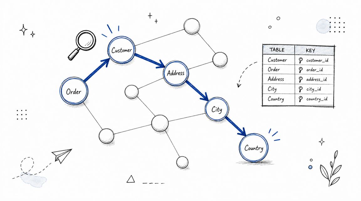
Most analytics problems aren't isolated rows. They're relationships. Customers connect to orders, orders connect to products, products connect to categories, and metrics connect to multiple source tables. Graph algorithms are the right fit whenever the challenge is traversing relationships instead of scanning a flat list.

A warehouse schema is often easier to reason about as a graph than as a pile of tables. Nodes represent entities. Edges represent joins, lineage, or dependency paths.

Here's the mental picture teams should use when debugging schema complexity:

How they help in analytics stacks

Graph traversal is useful when a system has to discover how tables relate without making a user define every join manually. In practice, that means finding the shortest join path between a customer table and a revenue table, tracing lineage from a dashboard metric back to raw events, or detecting circular dependencies in a transformation pipeline.

For a platform like Querio, graph algorithms become concrete. If a user asks a plain-English question, the system can't just understand the words. It also has to traverse the schema correctly. Breadth-first search is helpful for shortest paths. Depth-first search can expose dependency loops and fragile model design.

What usually goes wrong

Teams often overcomplicate graph modeling or ignore it completely. The first mistake creates maintenance overhead. The second creates broken joins and duplicate metrics. A simpler rule works better: model the relationships that matter for analysis, then cache the common paths.

• Map foreign keys clearly: Hidden join logic is one of the fastest ways to lose trust in self-serve analytics.

• Cache common traversals: Popular entity paths shouldn't be recomputed every time.

• Use graph logic for lineage: It's easier to audit a metric when you can trace every dependency.

A quick visual walkthrough can help if you want to explain graph traversal to non-engineers:

If your team keeps arguing about “which table is the source of truth,” graph thinking usually exposes the underlying issue. The relationships were never made explicit.

3. Dynamic Programming

Dynamic programming solves a specific kind of pain. You're computing something expensive, pieces of the work repeat, and your system keeps recalculating the same intermediate results. That's wasted time and wasted money.

Analytics teams run into this more often than they realize. Running totals, cohort retention, month-over-month growth, rolling averages, and nested KPI logic all contain overlapping subproblems. Dynamic programming works by storing those intermediate results instead of recomputing them. In classic computer science, that's one of the core foundational algorithm families because it reuses subproblem solutions rather than solving them again, as described in Princeton's discussion of algorithm analysis and cost trade-offs.

Where it pays off

In SQL-heavy environments, window functions are often the most practical expression of this idea. Functions like LAG, LEAD, and cumulative SUM let teams compute sequential metrics without procedural loops. Materialized views and precomputed aggregates apply the same principle at the system level.

For self-serve BI, this matters because users ask repeatable analytical questions. “How did retention change by signup month?” shouldn't trigger a fresh, fully expanded logic tree every time. A platform like Querio can cache intermediate metric states so users get answers without waiting on repeated warehouse work.

Cache the expensive middle step. That's usually where analytics systems lose responsiveness.

The trade-off is freshness. Cached results improve speed, but every cache introduces the question of when it should be invalidated. Teams that ignore that end up serving stale numbers with impressive latency.

4. Sorting Algorithms

Sorting seems basic until you look at how much analytics depends on order. Rankings, trend analysis, top-N reporting, pagination, percentile work, and time-series exploration all get easier once data is arranged predictably.

It also affects performance more than many teams expect. Sorted data can make downstream operations more efficient, especially range scans and certain merge-based operations. In day-to-day analytics work, that means faster dashboards and cleaner exploration when people ask for “top customers,” “latest activity,” or “biggest change since last month.”

Why sorted data changes everything

The business value is often simple. A sorted result is easier to interpret. But the technical value matters too. Once data is sorted by timestamp, account, or revenue, a lot of common operations become less chaotic. This is especially true in event streams and fact tables where “what happened next” is part of the question.

Use stable sorts when sequence matters, especially for time-series and transaction logs. Use database-native sorting when possible, because the query optimizer usually does a better job than hand-rolled application logic. And if the dataset won't fit in memory, design for external sorting instead of pretending the warehouse is a laptop.

• Pre-sort during ETL when helpful: It can make downstream analysis more predictable.

• Index columns users sort repeatedly: Common ordering patterns should be cheap.

• Avoid unnecessary sorts: Sorting large result sets “just in case” wastes compute.

A lot of bad dashboard performance comes from hidden sorts inside layered queries. If a report feels slow, inspect the ordering operations before you blame the warehouse.

5. Clustering Algorithms

A revenue team sees churn rising, but the usual segments are too blunt to explain it. Plan size, region, and industry show part of the picture. Instead, the split often comes down to behavior. Which accounts adopt quickly, which ones need repeated support, and which customers look healthy until usage drops.

Clustering helps teams find those patterns before formal labels exist. In analytics, that makes it useful for customer segmentation, product grouping, anomaly detection, and exploratory work where the question is still taking shape.

When clustering beats manual segmentation

Rule-based segments are still the right choice when the business needs clear operational buckets. Sales territory assignment, contract tier reporting, and lifecycle stage tracking usually need definitions that stay stable over time.

Clustering earns its keep when those fixed labels hide meaningful differences inside the same group. Two mid-market accounts can have the same ARR and industry but very different product behavior. One may use a broad set of features with low support demand. The other may log in often, adopt little, and generate repeated service tickets. Treating them as one segment leads to weak retention plans and generic reporting.

That matters in self-serve BI. Analysts and business users rarely ask for "run clustering." They ask why conversion changed, why NPS dropped in one cohort, or why a feature drives expansion for some customers but not others. A tool like Querio can support that workflow by surfacing natural groupings inside usage, support, or revenue data, then letting teams test whether those groups hold up in dashboards and follow-up queries. If you want a visual check on whether groups are separated, a scatter plot workflow in Tableau helps teams inspect cluster shape instead of trusting the model blindly.

Different clustering methods solve different business problems. K-means is often a practical starting point when you expect compact groups and need something fast enough for repeated analysis. Hierarchical clustering is useful when teams want to inspect nested relationships and decide later where to cut the tree. Density-based methods are better when outliers matter and clusters are irregular, which comes up often in fraud signals, operational incidents, and messy behavioral data.

The best clustering work changes a decision. If the output does not affect targeting, forecasting, onboarding, or support, it is just a tidy chart.

A few choices matter more than picking the trendiest method:

• Normalize features first: Variables on larger scales can overwhelm the rest and produce misleading groups.

• Choose features tied to action: Clusters based on columns nobody can influence rarely help the business.

• Test for stability: If small input changes create totally different clusters, do not build a strategy on top of them.

• Validate with operators: Customer success, sales, and product teams can tell you whether a segment is real or just mathematically convenient.

Clustering also has infrastructure implications. Segment discovery often runs across wide behavioral tables, repeated similarity calculations, and large intermediate datasets. Warehouses handle that work better when data is distributed predictably. For teams planning those pipelines, this guide on how hash partitioning improves load balancing is relevant because poor partitioning can slow the exploratory workloads clustering depends on.

6. Hash-Based Algorithms

Hashing is one of the least glamorous algorithm families and one of the most valuable. It powers fast lookups, deduplication, partitioning, and large-scale join strategies. If your analytics stack has to decide whether a value has been seen before or where a row belongs, hashing is probably involved.

The reason teams like hash-based approaches is simple. They turn messy comparison work into direct addressable structure. That's useful in warehouses, caches, distributed systems, and event pipelines.

Where hashing earns its keep

Hash joins are often the practical answer when large tables need to match on keys and sort-merge isn't the best fit. Deduplication pipelines also rely on hashing because exact row or key comparisons get expensive fast at scale. The same logic shows up in partitioning strategies for distributed compute.

For analytics products, the benefit is often invisible to the user but obvious in the experience. Queries resolve faster. Repeated entities collapse correctly. Data lands in predictable partitions. If your team is evaluating warehouse distribution strategies, this explainer on how hash partitioning improves load balancing is directly relevant to performance and workload spread.

• Choose hash functions for your data shape: Skewed keys create hot partitions and uneven workloads.

• Watch load factors: Hash tables degrade when they're overpacked.

• Use bloom filters where exclusion matters: They're useful for quickly ruling out non-matches before expensive work starts.

Hashing is not a silver bullet. It's excellent for exactness. It's much less helpful when users ask fuzzy, semantic, or relationship-heavy questions.

7. Machine Learning Algorithms

A revenue team sees churn rising, support volume climbing, and conversion rates slipping. Standard dashboards show the symptoms, but they do not estimate who is likely to leave next month, which tickets need urgent routing, or which accounts are most likely to expand. That is the point where machine learning becomes useful in analytics.

Machine learning algorithms help teams move from description to prediction and detection. In business settings, the question is rarely "Which model is most advanced?" The better question is "Which model fits the decision, the data quality, and the cost of being wrong?" A churn model with clear drivers may be more valuable than a complex model no one trusts enough to use.

Natural Resources Canada notes that classification methods are commonly grouped into supervised and unsupervised approaches, and that hybrid workflows can combine them, such as clustering first and then applying a classifier, in its overview of hybrid classification approaches. That matters in production analytics because useful systems are often multi-step workflows, not single-model exercises.

The practical families teams use

The main families are straightforward. Regression models forecast numeric values such as revenue, demand, or resolution time. Classification models assign labels such as "high churn risk" or "fraud review needed." Clustering groups similar records when labels do not exist yet. Dimensionality reduction helps compress wide datasets so analysts can model them faster and inspect patterns more clearly.

In self-serve BI, these algorithms also support the product experience, not just the end analysis. Natural-language understanding, metric suggestions, anomaly flags, and predictive prompts all depend on pattern recognition and ranking models. Querio applies that idea at the workflow level, where AI helps users move from a business question to a usable analysis. For a practical product view, see Querio's article on AI in data analytics.

The trade-offs are usually operational. Linear and tree-based models are easier to explain, easier to debug, and often faster to deploy. Neural networks can capture more complex patterns, but they demand more data, more tuning, and tighter monitoring. In analytics teams, that extra complexity only pays off when the business problem is large enough and the prediction target is stable enough.

A few selection rules save time:

• Use regression when the business action depends on a number: forecasting sales, estimating wait times, or predicting spend.

• Use classification when the action is threshold-based: approve, escalate, retain, investigate.

• Use interpretable models when stakeholders need to defend decisions: finance, operations, and customer-facing teams often need clear reasoning.

• Monitor drift after launch: product changes, seasonality, and policy updates can make last quarter's model unreliable.

Machine learning is a poor substitute for clear problem framing. If a rule, join, filter, or simple aggregation answers the question with less risk, use that first. The best analytics teams apply ML where uncertainty is real and where better predictions change decisions, not where a basic query already does the job.

8. Stream Processing Algorithms

Batch analytics tells you what happened. Stream processing helps you react while it's happening. That difference matters for fraud alerts, operational monitoring, product telemetry, marketplace activity, and live dashboards.

The algorithmic challenge is harsher here. A stream is continuous, potentially unbounded, and often messy. Events arrive late, out of order, or duplicated. The system has to work with limited memory and make decisions without repeatedly rescanning the full history.

What real-time systems must do differently

Windowing is one of the core ideas. Instead of aggregating over a fixed table, the system groups events by time or session boundaries. Watermarking helps handle late-arriving records. Backpressure control matters when the event rate spikes and downstream systems can't keep up.

For a self-serve analytics platform, stream processing can power near-live metrics and alerts. Users don't have to wait for overnight jobs to ask operational questions. They can track conversion flows, incoming events, or support activity as the data lands.

Real-time analytics fails less often because of math and more often because teams ignore event disorder.

A few choices matter early:

• Use session windows for behavior analysis: They match user activity better than rigid clock windows in many product cases.

• Test duplicate and late events: Streams in production are almost never clean.

• Be selective about exactly-once guarantees: They're valuable, but they also add complexity and cost.

If your business only reviews numbers once a week, streaming may be overkill. But if operational response time matters, batch pipelines won't be enough.

9. Approximate Query Processing Algorithms

Approximate query processing is one of the most practical ideas in modern analytics because it aligns with how people explore data. Early in analysis, most users don't need perfect precision. They need directional truth quickly enough to decide whether to dig deeper.

That makes approximate algorithms ideal for wide, large, and expensive datasets. Instead of scanning everything, the system can rely on sampling, sketches, or estimation structures to return a useful answer fast. Later, exact computation can validate the result.

When approximate answers are better than delayed exact ones

Interactive analytics lives or dies on response time. If a user asks five exploratory questions and every answer takes too long, the workflow collapses. Approximate methods preserve momentum. They're particularly useful for cardinality estimation, rough trend checks, and early-stage metric discovery.

This is also where business context matters. Approximation is a poor fit for final financial reporting. It's often a strong fit for exploration, product analysis, and operational triage. In self-serve systems, the best experience is usually hybrid: show a fast estimate first, then refine if the question becomes decision-critical. Querio's perspective on ad hoc queries fits this pattern because exploratory questioning works better when the system supports fast iteration.

• Use approximations for discovery: They help users narrow the search space.

• Escalate to exact answers for commitments: Board reporting and finance close need precision.

• Be transparent about estimated results: Users should know whether they're seeing a sketch or a full computation.

Teams often resist approximation because it sounds less rigorous. In practice, delayed certainty can be less useful than immediate direction.

10. Dimensionality Reduction Algorithms

A common analytics failure starts with a simple request. A team wants to explain churn, recommend the next best action, or group accounts by behavior. The warehouse has hundreds of columns, many of them correlated, sparse, or weakly useful. Querying is still possible, but pattern-finding gets slower, model quality drops, and analysts spend more time sorting signal from noise than answering the business question.

Dimensionality reduction cuts that problem down to size. These algorithms compress many variables into a smaller set that preserves the strongest structure in the data. PCA is the standard example. It projects data into components that explain the largest share of variation, which makes large feature sets easier to analyze, compare, and visualize.

The business value is practical. Fewer dimensions can reduce compute cost, improve clustering, and make similarity analysis more stable. It also helps teams see whether dozens of metrics are measuring the same underlying behavior.

In self-serve BI, this matters before a dashboard ever loads. A tool like Querio can use dimensionality reduction to identify which columns carry distinct information and which ones mostly repeat each other. That improves column selection, trims noisy inputs for downstream models, and gives AI-assisted analysis a cleaner starting point.

The trade-off is loss of interpretability. A principal component may be mathematically useful while being hard to explain to a sales leader or finance partner. t-SNE and UMAP can produce excellent visual groupings, but they are mainly exploration tools, not default replacements for business-facing features.

Use these methods with discipline:

• Scale features before PCA: Raw units can skew the result toward larger-value columns rather than more informative ones.

• Use reduction to improve analysis speed and structure: Keep the original variables available when stakeholders need a clear explanation.

• Choose the method based on the job: PCA works well for compression and preprocessing. t-SNE and UMAP work better for visual exploration of local patterns.

• Check what got lost: A smaller representation can remove noise, but it can also hide edge-case behavior that matters in fraud, support, or retention work.

Compression helps when wide data is the obstacle. It hurts when the discarded detail contains the business signal. The right choice depends on whether the goal is faster exploration, better preprocessing, or a result someone can defend in a meeting.

Comparison of 10 Algorithm Types

Build, Don't Just Query Turning Algorithms into Action

A revenue leader asks why pipeline slowed in one region. Operations wants the answer before the afternoon forecast call. Finance needs the same data reconciled to booked revenue. If every request still turns into a hand-built analyst ticket, the problem is no longer query speed. It is system design.

Knowing the main algorithm types changes how teams build analytics around that reality. Search handles fast retrieval. Graph algorithms expose relationships across customers, products, and accounts. Clustering finds segments that no one defined in advance. Stream processing catches changes while they are still actionable. Once teams classify requests by problem type, they can choose the right method, set realistic latency targets, and avoid forcing every business question through the same SQL-heavy workflow.

The older computer science categories still matter because they shape how analytics systems behave under load. Dynamic programming helps when repeated subproblems make brute force too expensive. Divide-and-conquer improves performance on large datasets. Hashing reduces lookup and join costs. In production, teams judge these choices on more than asymptotic efficiency. They care about accuracy, compute cost, failure tolerance, and whether the result can support a decision before the business window closes.

Algorithmic trading makes that trade-off easy to see. The right algorithm depends on the job. Execution algorithms such as TWAP, VWAP, and POV are built to control how orders hit the market, while strategy classes such as market making, arbitrage, statistical arbitrage, and trend-following target different return and risk profiles, as described in the CFTC discussion of algorithmic trading strategy types. The same principle applies in analytics. Choose for the objective function first, then for the data shape, latency requirement, and operational constraints.

Scale changes the standard. Quantified Strategies' review of algorithmic trading penetration and market projections reports that algorithmic trading accounts for roughly 60 to 75% of total trading volume across the U.S. equity market, European financial markets, and major Asian capital markets, while India is around 40%. The specific percentages matter less than the pattern. Once volume, complexity, and response-time pressure rise far enough, algorithmic infrastructure becomes part of the operating model.

Self-serve BI is moving in the same direction.

Teams do not need another dashboard layer that still depends on analysts to translate every vague request into the right logic. They need systems that apply search, graph traversal, clustering, dimensionality reduction, and machine learning patterns behind the scenes so commercial, finance, and operations users can work with warehouse data directly. Querio fits that model. It places AI coding agents on the data warehouse so technical and non-technical users can query, analyze, and build without routing each question through a central analytics queue.

Strong analytics teams do more than answer faster. They build environments where the right algorithm is already close to the question, and where better questions show up more often because the cost of exploration is lower.

If your team is stuck acting like a human API for the business, Querio is worth a look. It's designed to put AI coding agents directly on your data warehouse so people can explore, analyze, and build on company data with less analyst bottleneck and more self-serve capability.