Time Series Regression Analysis: Forecasting Growth & Impact

Your dashboard says signups are up. Finance wants next quarter’s forecast. Growth wants to know whether the campaign changed anything. Product wants to know if the onboarding redesign improved activation.

And your current answer is probably some version of: “It looks like a trend.”

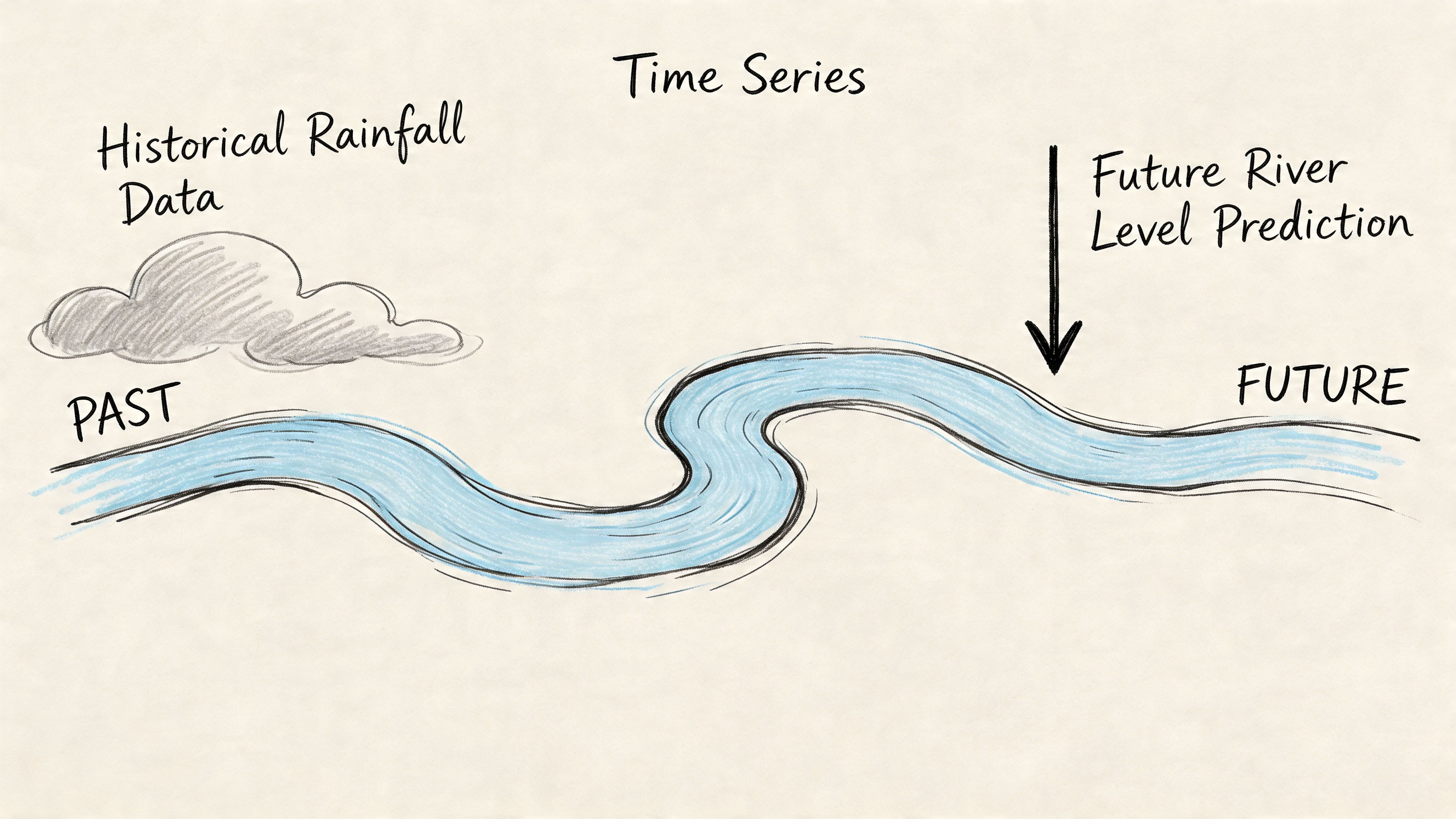
That’s the moment when it becomes apparent that ordinary reporting isn’t enough. A line chart can tell you what happened. A basic regression can tell you whether two variables moved together. But neither is built to handle what matters most in operating a startup: time.

Time changes everything. Yesterday affects today. Mondays don’t behave like Saturdays. Launches create temporary spikes. Pricing changes can shift the baseline. If your model ignores that structure, your forecast will usually look clean right up until the moment it fails in production.

Time series regression analysis is the practical middle ground between a spreadsheet guess and a research-paper-only method. It helps teams forecast future values, separate signal from noise, and estimate the impact of events using the natural order of observations over time. That’s why teams in finance, healthcare, retail, economics, and engineering use it for forecasting, trend analysis, and impact analysis, as described in this guide to regression analysis with time series data.

For a startup, the value is simple. You stop asking only “what happened?” and start answering “what’s likely next?” and “what changed the curve?”

Why Your Growth Forecasts Are Missing the Mark

A product manager exports weekly active users, drops them into a BI tool, adds a trend line, and calls it a forecast. It works for a few weeks. Then the next launch lands, seasonality kicks in, paid traffic shifts, and the estimate drifts far enough to affect hiring plans.

That pattern is common because many startup forecasts are built from tools designed for reporting, not for temporal dependency. A dashboard is good at slicing metrics by segment. It’s not good at understanding that this week’s usage may depend on last week’s usage, the month of the year, and a campaign that started two periods ago.

The hidden assumption in simple forecasting

Basic regression often assumes that rows are interchangeable. If you shuffle the order, the math still works. That’s fine for many cross-sectional problems. It breaks when the sequence itself carries meaning.

In time-based data, order isn’t decoration. It’s structure.

A signup on Friday doesn’t mean the same thing as a signup on New Year’s Day. Revenue during a feature rollout doesn’t mean the same thing as revenue during a quiet week. If you ignore timing, your model can confuse a temporary spike for a durable trend.

Time series regression analysis matters when the past helps explain the present, and when outside factors affect outcomes with a delay instead of instantly.

Why startup teams feel this pain first

Startups change their product, pricing, channels, and market positioning constantly. That means the data generating process is moving under your feet. Growth teams often rely on basic spreadsheet extrapolation or simple dashboard alerts because they’re fast. The cost is that those methods rarely separate trend, seasonality, and intervention effects cleanly.

A more practical approach is to treat forecasting and impact measurement as time-dependent questions. That’s where time series regression analysis becomes useful. It’s built for forecasting future values, analyzing trends, and measuring the effect of events by modeling how variables depend on their own past values and on present or past values of other variables, as outlined in this overview of sales forecasting concepts.

Here’s the startup version of the problem:

• Forecasting signups: Paid spend increased, but signups also rise every January.

• Measuring retention: A new onboarding flow launched, but a pricing change happened nearby.

• Planning inventory or support staffing: User demand rises in cycles that a straight-line model misses.

When teams say their forecasts are “off,” the issue usually isn’t effort. It’s model choice. They’re using tools that flatten time instead of respecting it.

Understanding Time Series Regression Fundamentals

A useful way to think about time series regression analysis is to picture a coffee shop trying to predict daily sales. Yesterday’s sales matter. Weather might matter. Day of week matters. Holiday weekends matter. And random weirdness still happens.

That’s a time series problem. You’re not just asking, “What affects sales?” You’re asking, “How do those effects play out over time?”

The four patterns you should look for

Most business time series are a mix of a few basic components.

• Trend means the long-term direction. If the coffee shop keeps adding loyal customers, sales may gradually rise over months.

• Seasonality means repeating patterns tied to a fixed calendar. Fridays may always be busier. December may always look different.

• Cycles are broader ups and downs that don’t follow a neat calendar. Think hiring booms, market slowdowns, or budget freezes.

• Residual noise is everything your model doesn’t explain. A nearby street closure. A one-off influencer mention. A payment outage.

If you skip this decomposition step, you’ll often build the wrong model for the wrong question.

What regression adds to the picture

A plain time series can show you the path of one metric over time. Regression adds explanatory variables. That lets you test whether outside factors influence the outcome.

For the coffee shop, the target might be daily revenue. Inputs could include temperature, promotion days, staffing levels, and the previous day’s revenue. For a SaaS product, the target could be weekly activations. Inputs might include email sends, paid spend, release dates, and lagged activation values.

That’s why time series regression analysis is so practical for product and growth work. It’s not only about extrapolating a line forward. It’s about linking business actions to movement in the metric.

Where people get confused

The biggest misunderstanding is thinking “time series” automatically means “fancy forecast.” It doesn’t. It starts with disciplined data structure.

You need observations collected at consistent intervals. Daily, weekly, monthly. Not “whenever someone exported a CSV.” If the cadence is messy, the signal gets harder to interpret.

You also need enough context to see recurring behavior. If you only have a short snapshot, a random bump can look like a meaningful pattern.

Practical rule: before fitting any model, ask whether your timestamp cadence matches the business decision cadence. Daily support staffing needs daily data. Quarterly planning probably doesn’t.

If you want a solid refresher on regression before layering in time, Aakash Gupta’s actionable guide to regression analysis is a useful companion. For a more time-focused walkthrough, this practical explanation of time series analysis helps connect the statistical ideas to business use.

A simple mental model

Think of time series regression like driving with both a windshield and a rear-view mirror.

• The rear-view mirror is your lagged history.

• The windshield is your forecast.

• The road signs are external variables such as campaigns, weather, or launches.

• The bumps in the road are noise, outliers, and shocks.

A good model doesn’t pretend the road is perfectly straight. It tries to capture the route well enough that you can make better decisions before the next turn.

Choosing Your Model A Guide to Common Approaches

Not every team needs every time series model. They need the right one for the decision at hand.

The wrong habit is starting with the trendiest tool. The better habit is starting with the business question. Are you building a baseline forecast? Estimating the effect of a launch? Explaining a recurring seasonal pattern? Handling many external variables?

That choice determines whether you should start with classical regression, ARIMA, Prophet, or a machine learning model.

Start with the simplest model that can fail honestly

A useful rule for startup teams is this: if a simple model can explain the process clearly, begin there. Complexity should earn its place.

Classical regression with time-based features is often enough for a first production model. You can include trend terms, weekday indicators, monthly seasonality, lagged values, and known external drivers. It’s interpretable, fast to debug, and easy to explain to finance or leadership.

ARIMA and related models become more useful when the series itself carries strong internal structure, such as autocorrelation and persistent trend behavior that ordinary regression doesn’t capture well.

Prophet is often attractive for teams that want a quicker path to business forecasting with clear calendar effects. Machine learning models become relevant when patterns are non-linear, the feature set is large, or the data frequency is high enough to support more flexible learning.

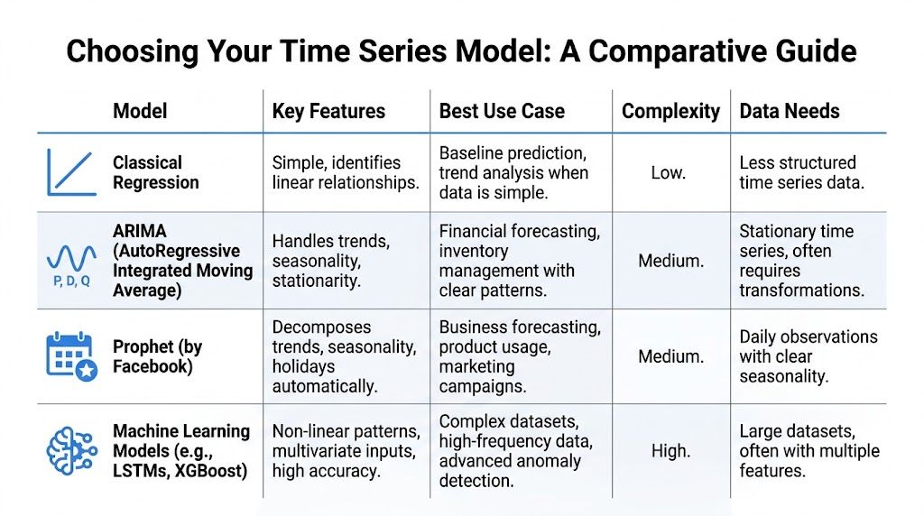
Comparison of Time Series Regression Models

Classical regression when you need clarity

Classical regression is the best place to start when stakeholders need to understand the “why” behind the prediction. You can say: weekday effects look like this, campaign periods look like that, and the prior week still matters after controlling for both.

That’s especially helpful in product and growth settings where the output needs to drive action, not just accuracy. If paid spend rises and a launch date variable is significant while holding seasonality constant, that’s a useful planning insight.

Use it when:

• You need explainability: Leadership wants to know what moved the number.

• You have external drivers: Spend, pricing, launches, or weather matter.

• You need a reliable baseline: You want to know whether a more advanced model is worth the added complexity.

ARIMA when the series remembers itself

ARIMA models are built for temporal memory. They’re useful when the present value is strongly shaped by prior values and prior errors.

The tradeoff is setup. ARIMA usually asks more from the analyst. You need to think carefully about stationarity, differencing, and whether seasonality needs its own treatment. But for inventory demand, financial-style series, or recurring operational metrics, that structure can be worth it.

Use it when:

• The series has clear autocorrelation

• You care about statistically grounded temporal structure

• You have enough historical data at consistent intervals

Prophet when the calendar drives behavior

Prophet is often chosen because it aligns with how business users think. Trend, seasonality, holidays. That mental model maps well to product usage, marketplace activity, and many sales-style problems.

It’s not magic. It still needs clean data and thoughtful validation. But it can get a team to a practical forecast quickly when daily observations and calendar effects dominate the pattern.

A strong fit includes metrics like:

• Daily active users with weekday swings

• Order volume around holidays

• Support volume with recurring weekly patterns

Machine learning when interactions get messy

Machine learning models shine when many variables interact in non-linear ways. For example, campaign effects might depend on device type, region, prior engagement, and time since signup. A tree-based model or sequence model may capture interactions that a simpler model won’t.

The catch is business usability. These models can be harder to debug, easier to overfit, and tougher to explain when a stakeholder asks why the forecast moved.

Don’t choose a model because it sounds advanced. Choose it because the business cost of being wrong justifies the added complexity.

A practical model selection heuristic

If you’re deciding fast, use this sequence:

1. Build a naive baseline using last period or rolling average logic.

2. Try classical regression with lagged features and seasonality indicators.

3. Move to ARIMA or SARIMA if residual structure still looks strongly time-dependent.

4. Use Prophet when calendar effects are dominant and you need a business-friendly workflow.

5. Use machine learning only after the simpler options have clearly left signal on the table.

This order forces discipline. It also makes debugging easier because each step teaches you something about the series.

What matters more than the model label

Teams often over-focus on the algorithm and under-focus on the operational fit. In practice, ask these questions:

• Can the team maintain it?

• Can someone explain the output in a planning meeting?

• Can the model absorb new data without heroics?

• Does it support intervention analysis, forecasting, or both?

That’s the core decision framework. The best model isn’t the most complex one. It’s the one your team can trust, update, and use to make decisions next week.

Your Practical Time Series Regression Workflow

Most forecasting projects fail long before modeling. They fail in data prep, time alignment, weak validation, or bad handling of missing values. A practical workflow keeps you from mistaking those avoidable issues for “model performance.”

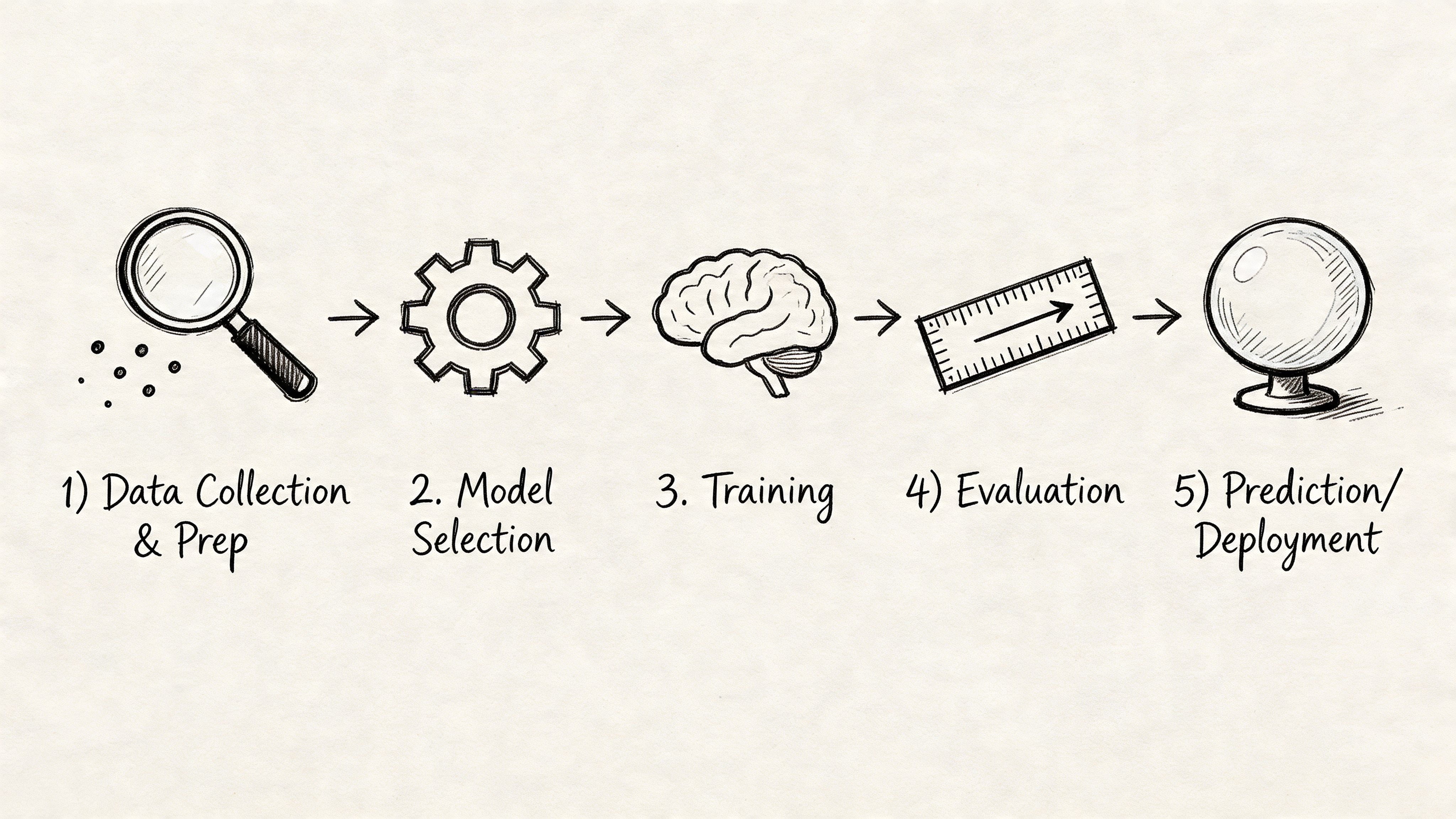
Step one get the data into a real time series shape

Time series regression analysis needs more than historical records. It needs records at a consistent interval over a meaningful stretch of time. Tableau’s explanation of time series analysis notes that effective analysis requires substantial data volume and that the goal is to capture the underlying signal rather than reproduce a specific historical event, as explained in this overview of time series analysis and forecasting.

For a startup, that usually means first fixing the warehouse extract.

Check these basics before anything else:

• One row per period: Daily means daily. Weekly means weekly. Don’t mix them.

• A trustworthy timestamp: Use one business definition of the period boundary.

• Stable metric logic: Don’t let “active user” mean one thing in January and another in March.

• Known interventions marked: Product launches, campaigns, pricing changes, outages.

A lot of confusion disappears when the dataset itself stops changing shape.

Step two plot the series before you touch a model

This sounds simple because it is. It’s also where many teams skip too fast to fitting.

Plot the target over time. Then plot it with obvious event markers. Then compare it by weekday, week, or month depending on cadence. You’re looking for rough trend, recurring cycles, unusual spikes, level shifts, and gaps.

If you’re mentoring a PM, I’d frame it like this: before asking the model to explain the business, make sure you can explain the picture.

Here’s a minimal Python setup:

import pandas as pd
import matplotlib.pyplot as plt

df = df.sort_values("date")
df = df.set_index("date")

df["signups"].plot(figsize=(10, 4), title="Daily Signups")
plt.show()

Step three build time-aware features

Raw timestamps rarely help on their own. The model needs features that represent temporal behavior.

Common features include:

• Lagged values: yesterday, last week, last month

• Rolling summaries: rolling mean, rolling max, rolling volatility

• Calendar indicators: day of week, month, holiday flags

• Intervention flags: campaign live, feature on, pricing version

• External regressors: spend, weather, inventory, traffic source mix

For example:

df["lag_1"] = df["signups"].shift(1)
df["lag_7"] = df["signups"].shift(7)
df["rolling_7"] = df["signups"].rolling(7).mean()
df["day_of_week"] = df.index.dayofweek

The value of notebooks over rigid dashboards often becomes apparent to many teams when interacting with systems that support Python directly on warehouse data. In such environments, iterating on lags, event flags, and diagnostics becomes possible without waiting for a custom BI setup. That’s the practical appeal of workflows like this SQL and Python demand forecasting approach.

Step four deal with missing values carefully

Missing data is one of the most underappreciated failure points in time series regression analysis.

A startup metric often goes missing for operational reasons, not random ones. Tracking changed. ETL failed. A metric wasn’t logged over a weekend. A region launched later than others. If you just drop rows, you can bias the pattern because time-adjacent observations and related entities are connected.

Missing periods aren’t just blank cells. In time series, they can distort trend, seasonality, and intervention estimates.

For time-series cross-section data, advanced multiple imputation methods are often better than listwise deletion or simplistic fill-ins. Verified background material notes that standard deletion can introduce severe bias, and advanced multiple imputation can reduce trend estimation errors by 20-50% in series with 30% missingness, based on the cited summary in the verified data. The practical lesson is straightforward: don’t default to dropping missing periods just because it’s easy.

A useful decision rule:

Step five check whether the series needs transformation

Some series are easier to model after transformation. If variance grows with scale, a log transform may stabilize things. If trend dominates and the model assumes a more stable process, differencing may help.

You don’t need to turn this into a PhD exercise. The point is to make the model learn the pattern, not the artifact.

A practical interpretation:

• If the line keeps drifting upward and residuals track that drift, the model may need trend handling or differencing.

• If variance gets wider as the series gets larger, consider a scale transformation.

• If weekly peaks repeat cleanly, seasonality terms likely matter more than another fancy algorithm.

Step six validate with time in the right direction

The most common validation mistake is random train-test splitting. That leaks the future into the past.

Time-aware validation respects chronology. Train on earlier periods. Test on later periods. Then roll the window forward and repeat. This mimics how forecasting works in practice.

train = df.loc[: "2024-06-30"]
test = df.loc["2024-07-01":]

features = ["lag_1", "lag_7", "rolling_7"]
X_train = train[features].dropna()
y_train = train.loc[X_train.index, "signups"]

X_test = test[features].dropna()
y_test = test.loc[X_test.index, "signups"]

Don’t just ask whether the model predicts well on average. Ask whether it fails in the periods you care about. Month-end. Peak season. Post-launch weeks.

A quick walkthrough can help if your team is newer to the tooling side:

Step seven inspect residuals like a skeptic

Residuals are the leftover errors after the model makes its prediction. If they still show visible patterns over time, your model is missing structure.

Look for:

• Autocorrelation: errors that clump by time

• Seasonal leftovers: regular spikes the model missed

• Intervention misses: sustained error after a launch or campaign

• Variance changes: errors getting larger in high-volume periods

If residuals still “remember” time, your model probably isn’t finished.

Step eight move from notebook to production

A production-ready forecast isn’t just code that ran once. It needs operating rules.

At minimum, define:

1. Refresh cadence based on the decision cycle.

2. Input checks for missing periods and metric drift.

3. Retraining trigger when error or residual behavior changes materially.

4. Fallback forecast if the main pipeline fails.

5. Output format that non-technical stakeholders can use.

The operational shift matters. Forecasting isn’t a one-time analysis deck. It’s a recurring business process.

Applying Time Series Regression in Product and Growth

Time series regression analysis merits the effort involved. It helps product and growth teams answer business questions that dashboards usually leave half-answered.

Did the launch change behavior or just coincide with noise

A product team launches a new onboarding flow. Activation jumps the following week. The easy story is “the redesign worked.” The harder question is whether the increase would have happened anyway because of seasonality, campaign spillover, or a broader traffic shift.

Segmented time series regression or intervention analysis is helpful. For effective intervention analysis, basic models need at least 12 pre- and post-intervention data points, while extensions such as ARIMA or SARIMA may require 50-100+ pre-intervention observations when seasonality or lagged effects matter, according to this segmented regression guidance for interrupted time series studies.

For startups, that constraint matters. Teams often want causal confidence from a short window. The model may not support it yet.

The campaign question growth teams ask every quarter

Growth launches a campaign and sales rise. Was it the campaign, the time of year, or both?

Time series regression gives you a better frame than before-and-after comparisons. You can include a campaign indicator, lagged performance, and seasonal controls. That helps estimate whether the campaign changed the level, the slope, or neither.

One caution matters a lot here. Standard models that ignore seasonality can bias the measured intervention effect by 15-30% in public health simulations, according to the same interrupted time series source. The startup translation is simple: if your business has weekly or monthly rhythms, don’t measure campaign impact with a flat baseline.

A spike after launch is not the same thing as an effect caused by launch.

Three practical startup use cases

• Forecasting demand for operations: Support volume, order count, or usage load often follows recurring patterns plus external drivers. A forecast helps staffing and infrastructure planning.

• Measuring pricing or packaging changes: Add an intervention variable and inspect whether the level shifts, whether the slope changes, or whether the change fades.

• Separating channel impact from underlying trend: Paid spend may lift short-term activity, but the underlying product trend may already be improving or weakening.

If you work in adjacent markets with highly variable transaction timing, it can help to study more unusual examples too. This write-up on Ethereum gas price prediction is a useful reminder that temporal forecasting problems often combine recurring patterns with sudden shocks. That’s not just a crypto issue. Product usage and acquisition costs can behave the same way.

What data you actually need for these decisions

The business question should determine the dataset.

For product impact analysis, collect:

• Target metric: activation, retention, conversion, usage frequency

• Intervention timing: release date, rollout window, experiment flag

• Confounders: campaigns, pricing changes, outages, major seasonality

• Stable cadence: daily or weekly, depending on user behavior

For growth forecasting, collect:

• Outcome metric: signups, qualified leads, subscriptions, sales

• Drivers: spend, impressions, channel mix, promo calendar

• Lagged history: enough to capture cycles and delayed response

If you need a simple business-facing example of how forecast outputs connect to sales planning, this sales forecasting example is a helpful companion to the more statistical approach here.

The real payoff

The value isn’t only a cleaner chart. It’s better operating decisions.

A PM can decide whether to roll out a feature more broadly. A growth lead can judge whether a campaign changed the baseline or only pulled demand forward. A founder can tell whether current momentum is durable enough to plan hiring against.

That’s the point of time series regression analysis in startups. It turns temporal data from hindsight into evidence you can act on.

From Reactive Reporting to Proactive Forecasting

Organizations often begin with dashboards because dashboards are easy to ship. The problem is that dashboards are reactive. They summarize the past. They rarely explain temporal structure well enough to support planning, intervention analysis, or credible forecasting.

Time series regression analysis changes the operating model. You structure the data by time, inspect trend and seasonality, create lagged and event features, validate in chronological order, and monitor residuals instead of trusting a one-off fit. That workflow is more disciplined than ad hoc reporting, but it’s also more practical than many academic treatments make it sound.

The fundamental shift is organizational. Product, growth, and data teams stop behaving like they’re waiting for an analyst to answer every “what happened?” question. They start building repeatable systems that answer “what’s likely next?” and “what changed the curve?”

That’s especially important for startups. Your roadmap, spend, and staffing decisions all depend on whether today’s movement is noise, seasonality, or a durable change. A better model won’t remove uncertainty. It will make uncertainty more legible.

Modern self-serve analytics tools can help if they let teams work directly with warehouse data, iterate in Python, and move from exploration to production without rebuilding the same logic across disconnected tools. That’s the practical path from reactive reporting to proactive forecasting.

If your team wants to build forecasting and impact analysis directly on top of warehouse data, Querio is one option to evaluate. It deploys AI coding agents on your data warehouse and supports notebook-based workflows, so analysts, product managers, and data teams can work on time series modeling, regression, and operational analytics in a more self-serve way.