Supply Chain Management
SQL and Python for AI Demand Forecasting
Use SQL for data prep and Python for modeling to build automated, scalable AI demand forecasts with feature engineering and validation.
SQL and Python are powerful tools for creating AI-driven demand forecasting systems that help businesses predict customer needs more accurately. SQL handles data preparation, cleaning, and enrichment directly from cloud data warehouses, while Python enables advanced modeling with libraries like Prophet and scikit-learn. Together, they streamline forecasting by automating workflows, reducing manual errors, and improving forecast accuracy.
Key Takeaways:
SQL: Ideal for extracting and cleaning historical data, filling gaps, and enriching datasets with external variables like holidays or weather.
Python: Used for feature engineering, advanced modeling, and validating forecasts with metrics like MAPE and RMSE.
Automation: Tools like Querio simplify the process by generating SQL and Python code, enabling scalable forecasting across SKUs.
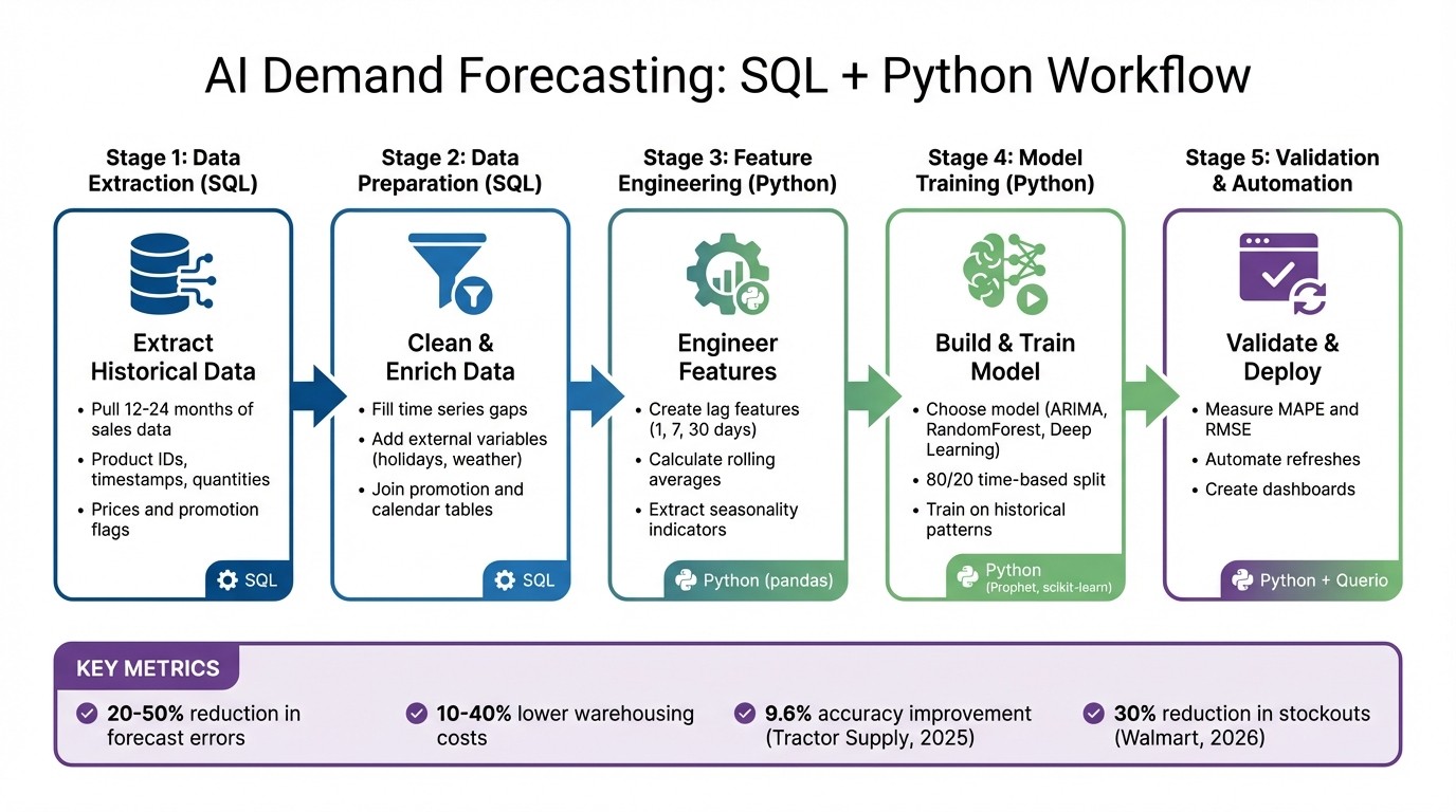
AI Demand Forecasting Workflow: SQL to Python Implementation Steps
Preparing Data with SQL
Extracting Historical Demand Data
To get started, pull key details like product IDs, timestamps, quantities sold, prices, and promotion flags from your sales table. Focus on data from the past 12–24 months to ensure you have a robust dataset. Make sure date columns follow a consistent format (e.g., YYYY-MM-DD). SQL window functions, such as LAG(), and rolling averages can help you uncover trends directly within your data warehouse. This approach is ideal for live data processing, keeping your workflow efficient and easy to update when refreshing forecasts weekly or monthly.
Once you’ve extracted the data, it’s crucial to address any inconsistencies or missing information that could undermine your model’s accuracy.
Handling Missing Data and Time Series Gaps
Gaps in time series data can throw off forecasts. To tackle this, SQL can create a complete date range and left-join it to your sales data. This allows you to fill gaps with either zero demand or the last known value. For instance, if no sales occurred on a holiday, filling that gap with a zero is far better than leaving it blank - it provides a clearer picture of demand patterns.
A real-world example: Tractor Supply Company improved their forecast accuracy by 9.6% in 2025 after implementing a real-time system that automated the handling of gaps and data updates [1]. Automating this process ensures your models always work with clean, continuous data during every refresh.
Once your dataset is complete, you can enhance it further by incorporating external variables.
Adding External Variables
External factors can have a significant impact on demand. Variables like holidays, weather, and marketing campaigns often drive sales trends. Use SQL joins to enrich your historical demand data by linking it with external datasets. For example, connect a calendar table marked with holidays or a promotions table that includes discount percentages and advertising spend.
Variable Category | SQL Variables to Include | Purpose |
|---|---|---|
Temporal | Holidays, Weekday/Weekend flags, Seasonality index | Identify cyclical demand changes |
Marketing | Promotion flags, Discount %, Ad Spend | Assess the influence of campaigns |
Product | Price, Category, SKU | Monitor price sensitivity and stock levels |
External | Weather (Temp/Precipitation), Market Trends | Factor in environmental and macro trends |
Data Cleaning and Feature Engineering in Python
Loading Data from SQL to Python
After enriching your data in SQL, the next step is to load it into Python for modeling. The pandas.read_sql() function is your go-to tool for this, allowing you to bring data directly into a DataFrame by connecting to your data warehouse through SQLAlchemy engines or ADBC drivers. This works seamlessly with platforms like Snowflake, BigQuery, or Postgres [2][4].
For massive datasets spanning years, consider using the chunksize parameter to load data in manageable batches. Alternatively, configure SQLAlchemy with stream_results=True to enable server-side cursors, which stream rows on demand [2][3]. While loading, you can use the parse_dates argument to automatically convert date columns into Python datetime objects [2]. Once your data is efficiently loaded, you can move on to cleaning and preparing it for feature engineering.
Cleaning and Preparing Data
Once your data is extracted and enriched, the next step is refining it in Python to ensure it’s ready for modeling. Start by inspecting your DataFrame with commands like df.info() and df.isnull().sum() to check data types and identify missing values [5]. Sorting your DataFrame by product identifier and date is critical at this stage - it preserves the temporal order, which is essential for building lag features without introducing data leakage [6].
When handling missing values, it’s important to think strategically. Use df.fillna() to fill gaps with zeros (for days with no sales) or the last known value, depending on your specific business needs [5]. However, hold off on dropping rows with df.dropna() until after creating lag features, as the shifting process naturally introduces NaN values at the start of each product’s time series [6].
Creating Forecasting Features
Feature engineering is where raw data is transformed into meaningful signals for forecasting. While SQL window functions are great for basic aggregations, Python’s .shift() and .rolling() methods let you create more nuanced features. Start by generating lag features with .shift() grouped by product ID. Common lags include 1-day, 7-day, and 30-day intervals, capturing immediate and weekly patterns. Be sure to apply these before rolling calculations to ensure your model only uses data available up to the prediction point [6].
Next, use .rolling(window).mean() to calculate rolling averages, such as 7-day or 30-day moving averages. These help smooth out noise and highlight short-term trends [6]. You can also extract seasonality indicators from your datetime column with .dt.dayofweek and .dt.month, helping your model recognize weekly and monthly patterns [6].
"Forecasting is not about guessing tomorrow. It's about using yesterday intelligently." [6]
For even more advanced seasonality and holiday effects, libraries like Prophet can tackle overlapping patterns and sudden spikes that simpler features might miss [1]. A notable example: in 2025, Tractor Supply Company implemented a real-time forecasting solution that automated both feature engineering and data handling. This change improved their forecast accuracy by 9.6% and reduced stockouts [1]. These engineered features lay the groundwork for building and training a reliable forecasting model.
Building and Validating Your Forecasting Model
Choosing the Right Model
The model you choose should align with the complexity of your demand patterns and the data you've gathered. For products with stable, predictable demand, ARIMA (Autoregressive Integrated Moving Average) is a reliable option. It handles seasonal patterns effectively and requires minimal programming effort. However, when dealing with products influenced by external factors - like promotions, weather changes, or local events - RandomForestRegressor can better capture these non-linear relationships. For businesses managing thousands of SKUs with intricate interactions, deep learning tools like TensorFlow or PyTorch may be necessary. For example, in 2026, Target uses AI for over 40% of its SKUs, generating billions of predictions weekly to optimize its assortments. Adapting your model to match product behavior - such as using separate models for stable versus highly seasonal items - often leads to better results [7].
Training and Testing the Model
Once you've chosen a model, the next step is training and testing to evaluate its performance under realistic conditions. Time series forecasting requires a chronological data split rather than a random one. A common approach is to use the first 80% of time-ordered data for training and the remaining 20% for testing, simulating future scenarios. Ensure your data is sorted by date (and product ID, if applicable) to maintain the integrity of lag features. Incorporate the features you previously engineered during training.
For instance, in early 2026, Walmart used AI-powered demand forecasting that combined local weather and event data with sales figures. This approach improved forecast accuracy and reduced stockouts by about 30%. Similarly, Idaho Forest Group cut their forecasting time from over 80 hours to under 15 hours by iteratively refining their models and feature sets [7].
Validating Model Accuracy
After training your model, it's crucial to validate its accuracy thoroughly. Use multiple metrics to assess performance. Mean Absolute Percentage Error (MAPE) helps measure errors relative to overall demand, while Root Mean Squared Error (RMSE) penalizes larger mistakes more heavily. Additionally, tracking forecast bias can reveal whether your model consistently over- or under-predicts demand.
AI-driven demand forecasting has been shown to reduce errors by 20–50% and lower warehousing and logistics costs by 10–40%. To sustain accuracy, set up feedback loops that compare forecasts with actual sales data and initiate retraining when discrepancies exceed acceptable limits. For greater transparency, tools like SHAP (Shapley Additive Explanations) or LIME can explain which factors - such as weather, promotions, or historical demand - carry the most weight in your predictions [7].
Scaling and Automating Forecasting with Querio
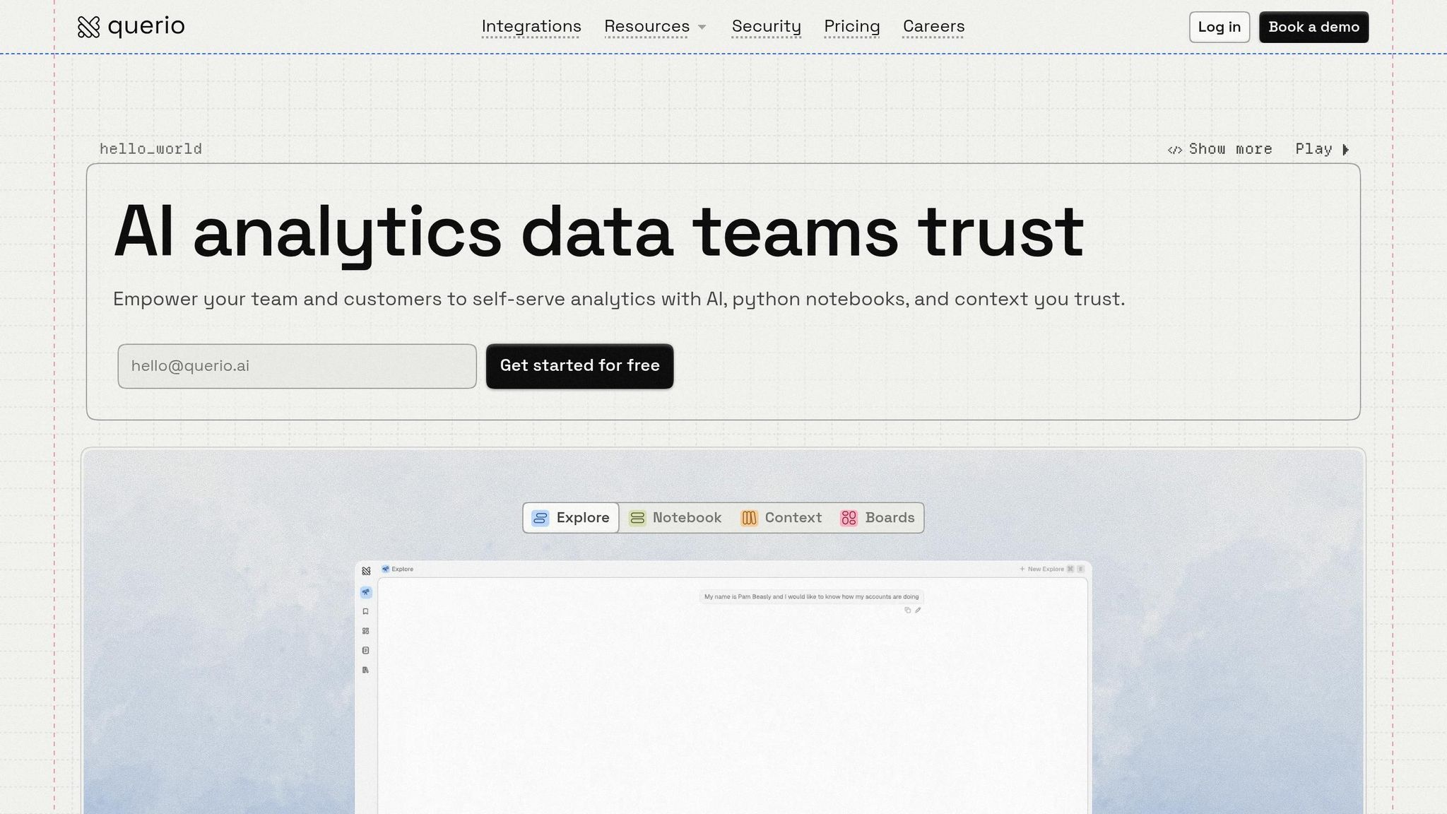
Using Querio for SQL and Python Code Generation
Once you've built a demand forecasting model, scaling it across hundreds - or even thousands - of SKUs can feel daunting. Querio simplifies this process by automating code generation, so you don’t have to rewrite queries for every product category. Instead of manually crafting complex SQL, you can ask natural language questions like, "What was the average demand for Product X across regions and product lines last quarter?" Querio generates clear, reliable code that works seamlessly with your live data warehouse, whether you’re using Snowflake, BigQuery, or Postgres.
This automation speeds up testing and iteration. For example, if you want to see whether adding variables like competitor pricing or social media mentions improves forecast accuracy, you can ask follow-up questions in plain English. Querio keeps the generated code transparent and reviewable, so it’s never a black box. This is critical when presenting forecasts to teams like supply chain or finance, where credibility and clarity matter.
Building Dashboards and Reports
Querio doesn’t stop at code generation - it also makes creating dashboards and reports much easier. Its notebook-based analytics environment allows you to build and refine demand forecasting models without juggling multiple tools. You can extract data with SQL, switch to Python for feature engineering and model training, and document your assumptions - all within the same workspace. Once your model is ready, Querio helps you turn it into a reusable dashboard tailored to different stakeholders.
For example:
Supply chain teams get granular forecasts by SKU and location, including lead time recommendations.
Finance teams see aggregate forecasts by product line, along with potential revenue impacts.
Executives view high-level trends with explanations for any variances.
Querio also automates report scheduling, ensuring forecasts refresh on a set schedule. Imagine a retail company setting weekly updates every Sunday evening - store managers would always have the latest demand predictions before finalizing inventory orders for the week ahead. This level of automation is a game-changer when handling hundreds of SKUs across multiple locations, where manual updates would be overwhelming.
Ensuring Accuracy and Consistency
After automating your forecasts and building dashboards, maintaining consistent metrics becomes essential. Querio addresses this with a shared context layer that serves as a single source of truth for your forecasting logic. Data teams define key metrics once - for instance, how "demand" is calculated (units sold, revenue, or orders), which time periods to include, how to handle returns or cancellations, and which external factors (like seasonality or promotions) are standard. This prevents conflicting forecasts caused by differing interpretations of the same metric, a common issue when scaling analytics across teams.
For example, you might decide that "Q2 demand" always excludes the first three days of April due to scheduled system maintenance. Or you might define "adjusted demand" to account for stockouts. These definitions are applied consistently across all analyses and dashboards. Querio's live, read-only connection ensures forecasts are based on up-to-date data. If a major customer places a large, unexpected order, that transaction will immediately reflect in your next forecast refresh. This alignment - from data extraction in SQL to model development in Python - ensures every step of your forecasting process stays consistent and reliable within your broader business intelligence strategy.
Conclusion
Key Steps Recap
Creating an AI-powered demand forecasting system using SQL and Python doesn’t have to be complicated. Start by extracting and cleaning historical demand data, then move on to feature engineering and model validation. Once the model is ready, automate the entire process. This approach ensures a smooth transition from raw data to actionable insights by leveraging SQL’s speed for data handling and Python’s advanced modeling tools - all in one streamlined workflow.
Benefits of Using Querio
Querio simplifies this process by turning a manual, time-heavy workflow into an automated and efficient system. Instead of managing countless SQL queries for various SKUs or juggling different tools for data processing and modeling, Querio allows you to ask questions in plain English. It generates inspectable SQL and Python code instantly, saving time and reducing errors. Plus, the shared context layer ensures that all teams work with the same definitions for metrics like "demand", eliminating inconsistencies across departments.
With live connections to platforms like Snowflake, BigQuery, or Postgres, your forecasts are always based on the most current data - no need for manual exports or dealing with outdated snapshots. This automation not only improves forecast accuracy and inventory management but also ensures consistency across your organization. With these tools in place, you’re set to refine and fully operationalize your forecasting model.
Next Steps
The next stage is to operationalize your forecasting system further. Automate model retraining and set up alerts for any performance issues to prevent model drift as customer behavior evolves [1]. Querio’s AI-native workspace simplifies this by handling code generation, maintaining metric definitions, and scheduling automated reports. This allows you to focus on enhancing your forecasting logic instead of worrying about infrastructure. Try Querio’s free trial to see how natural language queries and automated Python workflows can streamline your demand forecasting process.
Build a Demand Forecasting ML App: Python Data Science
FAQs
How much history do I need for demand forecasting?
When determining how much historical data to use, it really boils down to your business's nature, seasonality, and how far into the future you're forecasting. For markets that are relatively stable, 3–5 years of data is often sufficient. However, if you're operating in a fast-evolving industry, more emphasis should be placed on recent data to capture current dynamics.
It's important to choose a timeframe that mirrors present trends and seasonal shifts while steering clear of outdated information that no longer reflects reality. Tools like Querio can be incredibly helpful, as they analyze live, up-to-date data to keep your forecasts as accurate as possible.
Should I fill missing days with zeros or last values?
When deciding how to handle missing data, consider your dataset and modeling approach. For non-operational days, like weekends or holidays, filling gaps with zeros can accurately reflect no demand. For irregular gaps, such as those caused by data collection issues, using the last observed values (forward fill) helps maintain existing trends. Always ensure your choice aligns with your business context to keep forecasts reliable and avoid skewing trends or seasonal patterns.
How do I avoid data leakage with lag features?
When building lag features for demand forecasting, it's crucial to avoid data leakage by ensuring that the lagged data only reflects information available at the time of prediction. This means shifting the target variable backward in time and relying solely on past data. For instance, if you're forecasting today's sales, you should only include sales data from prior days in your model.
Additionally, pay close attention to missing values introduced during the lagging process. Proper handling of these gaps is essential to preserve the accuracy and reliability of your forecasts.
Related Blog Posts


