How to Handle Missing Data in Python: A 2026 Guide

Most advice on how to handle missing data starts with a shortcut: drop the rows, fill with the mean, move on. That advice is popular because it's fast, not because it's safe.

In practice, missing values are often telling you something about the system that produced the data. A survey field might be blank because a user skipped a sensitive question. A product metric might disappear only on certain devices. A warehouse column might be null because one upstream job failed for one customer segment. If you erase that pattern too early, you can clean your dataset and damage your analysis at the same time.

The production mistake isn't just bad imputation. It's treating missingness as a clerical problem instead of a modeling problem. The right workflow starts with diagnosis, chooses a strategy based on the mechanism behind the gaps, and ends with validation that the filled data still looks like the original data in ways that matter.

Table of Contents

• Beyond Mean Imputation Why Your Default Fix Is Flawed

• Diagnose the Damage What Kind of Missingness Do You Have

  • Read the mechanism before you fill anything

  • Use Python to inspect patterns, not just counts

• The Decision Framework When to Drop Impute or Model

  • Drop only when the loss is cheap and the bias risk is low

  • Impute when the variable matters and you can defend the filled values

  • Model the missingness when the gap is informative

• Hands-On Imputation Techniques in Python

  • Start with simple baselines

  • Use KNN when local similarity is real

  • Use MICE when one filled dataset is not enough

• The Last Step Validating Your Imputation

  • Compare summaries before and after

  • Plot the shape, not just the average

• Production and Warehouse Considerations for Data Teams

  • Keep the logic close to the warehouse

  • Version the method, not just the output

Beyond Mean Imputation Why Your Default Fix Is Flawed

Mean imputation is attractive because it's one line of code. It's also one of the easiest ways to flatten a variable until it no longer behaves like the thing you measured.

The problem isn't only statistical purity. It's operational damage. Mean and median fills can shrink variance, distort the shape of the distribution, and hide the fact that the missingness itself may carry signal. Tree-based algorithms such as decision trees and random forests can often handle missing values directly by splitting on available features, which means pre-imputing every column is often unnecessary in modern pipelines, as noted in the VA overview of missing data methods.

A mid-level analyst usually learns "clean the nulls before modeling." A stronger habit is: ask what the nulls mean before changing them.

Practical rule: If you can't explain why a value is missing, you shouldn't be confident about how to fill it.

This is also why missing-data handling belongs inside a broader quality workflow. Teams working on ensuring data quality for AI training already know that null handling, schema checks, drift checks, and annotation quality aren't separate problems. They're connected failure modes in one pipeline.

Common defaults fail in different ways:

• Dropping rows: Safe only in narrow cases. Otherwise you lose observations and can bias the sample.

• Mean filling numeric fields: Fast, but it pushes values toward the center and can erase real spread.

• Mode filling categorical fields: Useful as a baseline, but it can invent a false majority pattern.

• Single regression imputation: Better aligned with observed relationships, but it can be too optimistic if it doesn't carry uncertainty forward.

If you've ever felt that manually cleaning data becomes messy long before modeling starts, that's because it does. The operational reasons are well captured in this piece on what makes manually cleaning data challenging.

The mindset shift is simple. Missing data isn't dirt on the floor. It's evidence. Sometimes you fill it. Sometimes you model around it. Sometimes you preserve it on purpose.

Diagnose the Damage What Kind of Missingness Do You Have

Missing-data strategy starts with mechanism. If you don't identify the mechanism, your imputation choice is mostly guesswork.

Read the mechanism before you fill anything

Statisticians use three labels that matter in practice:

• MCAR, Missing Completely At Random
  Values are missing for reasons unrelated to observed or unobserved data. A logging glitch that blanks a few rows at random is the standard example.

• MAR, Missing At Random
  Missingness depends on data you do observe. A customer-income field might be missing more often for one region or one acquisition channel, but within those groups the actual missing value isn't driving the gap directly.

• MNAR, Missing Not At Random
  Missingness depends on the missing value itself or on something unobserved. Salary may be missing more often for high earners because they avoid disclosure. That's not a nuisance. That's part of the behavior.

The distinction matters because complete case analysis is only asymptotically unbiased under MCAR, while multiple imputation is designed for settings where data are MAR, according to Statistical Horizons on missing data methods.

In applied work, you usually don't prove the mechanism. You infer it from pattern, domain knowledge, and failure modes in the data pipeline.

When nulls cluster by segment, time, workflow step, or device type, you aren't looking at random dirt. You're looking at process behavior.

If your data sits inside a regulated or operationally messy domain, you'll often see this in CRM and operational records. That's why resources on banking CRM data cleansing are useful reading even outside banking. They force you to think about upstream process issues instead of treating every blank cell as a math problem.

Use Python to inspect patterns, not just counts

Most analysts begin with isna().sum(). That's necessary, but it's not enough.

Start with a missingness profile.

import pandas as pd

df = pd.read_csv("data.csv")

missing_counts = df.isna().sum().sort_values(ascending=False)
missing_pct = (df.isna().mean()).sort_values(ascending=False)

summary = pd.DataFrame({
    "missing_count": missing_counts,
    "missing_fraction": missing_pct
})

print(summary.head(20))

Then visualize the pattern.

import missingno as msno
import matplotlib.pyplot as plt

msno.matrix(df)
plt.show()

msno.heatmap(df)
plt.show()

msno.bar(df)
plt.show()

What you're looking for:

• Column clusters: Two fields go missing together, which often points to one broken upstream source.

• Time concentration: Nulls spike during one release window or one ingestion outage.

• Segment concentration: One customer type, geography, or product tier has systematically more gaps.

You can also create explicit missingness indicators and test whether they're associated with observed variables.

for col in ["income", "tenure", "credit_limit"]:
    df[f"{col}_missing"] = df[col].isna().astype(int)

print(df.groupby("region")[["income_missing", "tenure_missing"]].mean())
print(df.groupby("channel")[["income_missing", "credit_limit_missing"]].mean())

If the probability of missingness changes by observed group, MAR becomes more plausible than MCAR. If no observed variable explains the pattern but domain knowledge says the missing value itself likely drives the absence, treat MNAR as a live risk.

Tree-based models also give you a practical option here. Because decision trees and random forests can work with available features rather than requiring blanket pre-imputation, they can be a useful diagnostic baseline when you're unsure whether aggressive filling is helping or hurting.

For a stronger exploratory workflow around this stage, use the same habits you would use in general exploratory data analysis. Nulls are part of EDA, not a preprocessing footnote.

The Decision Framework When to Drop Impute or Model

The biggest mistake is treating imputation as the default. It is only one option, and in many real datasets it is the wrong first move.

After you identify the missingness pattern, make a deliberate choice among three paths: drop, impute, or model the missingness itself. The right answer depends less on textbook categories and more on what will break your analysis, your model, or your downstream decisions.

Drop only when the loss is cheap and the bias risk is low

Deleting rows or columns is fine when the missingness is plausibly random, the data loss is small, and the removed field is not carrying business-critical signal.

That standard is stricter than it sounds. A column with 8 percent nulls can still be too important to drop if those nulls are concentrated in high-value customers, one underwriting channel, or one release period. In production work, I treat deletion as a controlled simplification, not a cleanup habit.

Use deletion when:

• the field is peripheral to the question you are answering

• the missing records are few and look similar to the retained sample

• you need a fast exploratory baseline before building a better pipeline

Avoid deletion when missingness is tied to eligibility, behavior, risk, compliance, or the target itself.

Impute when the variable matters and you can defend the filled values

Imputation earns its place when the variable is useful, other features contain enough signal to estimate it, and you are willing to check whether the fill changed the shape of the data.

That last part gets skipped too often. Filling nulls is easy. Proving you did not flatten variance, create fake modes, or shift relationships between variables takes more work.

The practical ladder looks like this:

• Simple fills such as mean, median, or mode are baseline methods. They are fast, stable, and easy to productionize.

• KNN or regression-based imputation uses relationships across features and often gives more realistic values than naive fills.

• Multiple imputation is better for inference because it reflects uncertainty instead of treating estimates as observed truth.

MICE is often a strong choice for analytic work where preserving uncertainty matters, but it also adds complexity, runtime, and diagnostic burden. In practice, I would rather see a team run median imputation plus serious validation than use MICE mechanically and never check whether the completed data still resembles the original observed distribution.

If you need a broader implementation workflow for this kind of feature preparation, this guide on using Python for data analysis in production-style workflows is a useful companion.

Model the missingness when the gap is informative

This path gets ignored in a lot of tutorials, even though it often matters more than the imputation method itself.

A missing value can be signal. Income may be absent because applicants with volatile earnings skip the field. A lab result may be missing because healthier patients were never tested. In those cases, forcing a filled value into the column without preserving the fact that it was missing throws away useful information.

A practical pattern is to add a missingness flag before imputation, or keep an explicit "missing" category for categorical fields when that absence has operational meaning. Zest AI discusses this approach in its overview of methods for dealing with missing data, and the broader point is sound: when missingness correlates with the outcome, models often benefit from retaining that signal instead of hiding it.

Do not add flags blindly. Test them.

Here is a framework that works well in practice:

A simple decision rule helps. For predictive work, compare models with and without missingness indicators, then inspect whether the winning approach also preserves the underlying feature distributions. For inferential work, choose the method that makes the weakest unrealistic assumptions and gives you a credible story about uncertainty, sample bias, and distributional distortion.

Hands-On Imputation Techniques in Python

The fastest way to ruin a dataset is to fill every null with a single number and call it cleaned. Python makes imputation easy. It does not make it safe. The useful pattern in practice is to start with a cheap baseline, test stronger methods where the data supports them, and keep an eye on whether the filled values still look like the original feature.

Start with simple baselines

Median and mode imputation still have a place. I use them as control methods because they are fast, easy to reproduce, and stable in pipelines. They are also the quickest way to see whether a more complex method is earning its extra complexity.

import pandas as pd
from sklearn.impute import SimpleImputer

df = pd.read_csv("data.csv")

num_cols = ["age", "income", "tenure"]
cat_cols = ["plan_type", "region"]

# pandas baseline
df["income_median"] = df["income"].fillna(df["income"].median())

# scikit-learn baseline
num_imputer = SimpleImputer(strategy="median")
cat_imputer = SimpleImputer(strategy="most_frequent")

df[num_cols] = num_imputer.fit_transform(df[num_cols])
df[cat_cols] = cat_imputer.fit_transform(df[cat_cols])

Create missingness flags before the fill, not after it. That keeps the model from losing information that may matter.

for col in num_cols + cat_cols:
    df[f"{col}_was_missing"] = df[col].isna().astype(int)

That pattern works well for production features, especially when you need a straightforward pipeline that teammates can debug six months later.

If you want the broader context for where imputation fits in feature prep, this guide on how to use Python for data analysis is a useful companion.

Use KNN when local similarity is real

KNN imputation can produce more believable values than a global fill because it borrows from nearby rows. The catch is that "nearby" has to mean something. If your features are on wildly different scales, or half the matrix is sparse, KNN often looks smarter than it is.

from sklearn.impute import KNNImputer

features = ["age", "income", "tenure", "spend_score"]

knn_imputer = KNNImputer(n_neighbors=5)
df[features] = knn_imputer.fit_transform(df[features])

KNN is a reasonable choice when rows cluster in a way your feature set captures. Customer profiles, sensor readings, and repeated behavioral patterns often fit that description. Standardize numeric inputs first if scale differences are large, and be careful with high-cardinality encoded categoricals because they can make distance calculations noisy.

I usually compare KNN against median fill on three things: downstream model performance, runtime, and whether the imputed feature keeps a plausible spread instead of collapsing toward the middle. That last check gets skipped often, and it is where weak imputations get exposed.

A stronger option for many tabular datasets is iterative imputation, where each feature is predicted from the others in a repeating sequence. That tends to preserve multivariate structure better than one-column-at-a-time rules, although it costs more to run and tune.

Here's a short walkthrough if you want a visual explanation before implementing it:

Use MICE when one filled dataset is not enough

For analytical work, a single deterministic fill is often too neat. MICE generates several plausible completed datasets, which gives you a better handle on uncertainty than pretending each missing value had one obvious answer.

A practical implementation in Python can use miceforest.

import pandas as pd
import miceforest as mf

df = pd.read_csv("data.csv")

kernel = mf.ImputationKernel(
    data=df,
    save_all_iterations=True,
    random_state=42
)

kernel.mice(5)

completed_0 = kernel.complete_data(dataset=0)
completed_1 = kernel.complete_data(dataset=1)
completed_2 = kernel.complete_data(dataset=2)
completed_3 = kernel.complete_data(dataset=3)
completed_4 = kernel.complete_data(dataset=4)

The code is short. The judgment calls are not.

Match the imputation model to the variable type. Keep useful predictors in the imputation set instead of stripping the matrix down too early. Inspect whether the completed datasets remain plausible by segment, not just in aggregate. A method can look fine on the full column and still distort the distribution for high-value customers, recent cohorts, or rare categories.

That distribution check matters more than many tutorials admit. If the filled values flatten tails, erase skew, or weaken real correlations, the model may still train but the data no longer reflects the process you were trying to measure.

For warehouse-centered teams, notebook-based workflows make this easier to operationalize. pandas, scikit-learn, miceforest, and warehouse-native notebook environments can support the same logic. Querio is one example of a system that runs custom Python notebooks directly on warehouse data, which helps teams keep imputation code and post-fill validation close to governed source tables instead of scattering logic across local machines.

The Last Step Validating Your Imputation

Most tutorials stop too early. They show how to fill nulls, then move straight to modeling. That's where a lot of quiet damage gets introduced.

Validation is the difference between "the code ran" and "the data still means what we think it means." That step is widely skipped even though it catches obvious failures. According to Esri on dealing with missing data, 42% of imputed datasets in machine learning pipelines show significant skewing or flattening of histograms post-imputation, yet only 12% of published tutorials explicitly compare mean, standard deviation, and histogram shape before and after filling.

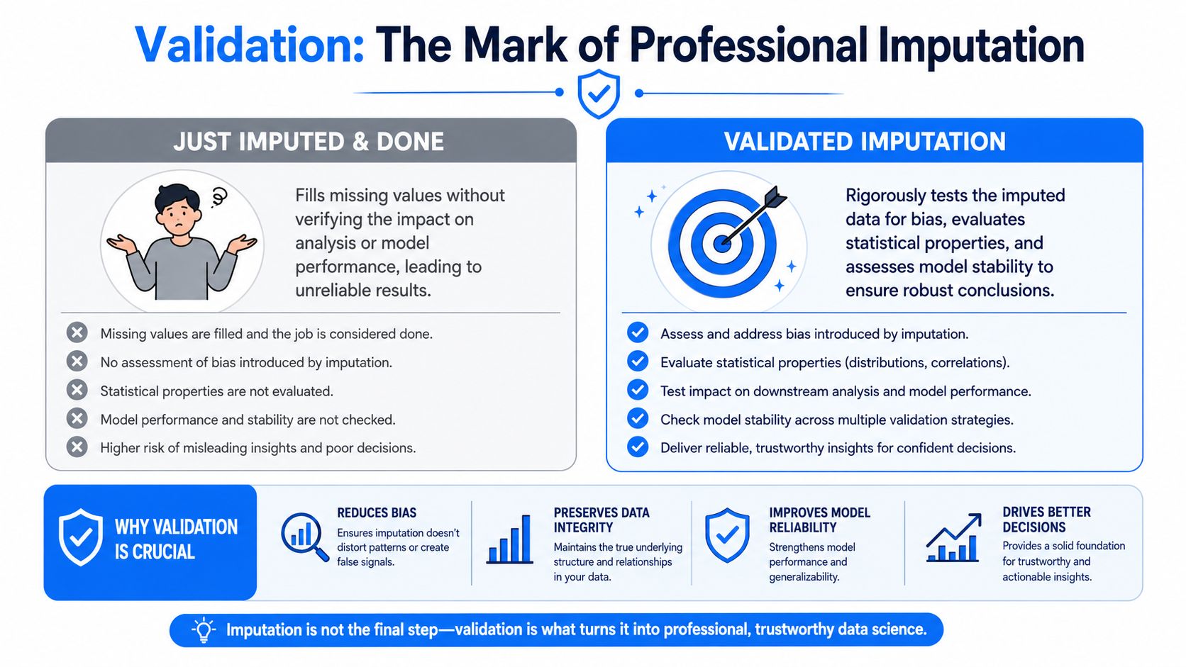
Compare summaries before and after

Start with a side-by-side summary on the original observed values versus the post-imputation column.

import pandas as pd

def compare_stats(original_series, imputed_series):
    observed = original_series.dropna()
    return pd.DataFrame({
        "observed_only": [
            observed.mean(),
            observed.std(),
            observed.min(),
            observed.max()
        ],
        "after_imputation": [
            imputed_series.mean(),
            imputed_series.std(),
            imputed_series.min(),
            imputed_series.max()
        ]
    }, index=["mean", "std", "min", "max"])

print(compare_stats(df["income_original"], df["income_imputed"]))

You are not looking for identical numbers. You're looking for suspicious shifts. If standard deviation collapses after mean filling, that isn't harmless cleanup. It means you've changed the variable's spread.

A fast imputation method that changes the shape of a key feature can hurt more than leaving some values missing.

Plot the shape, not just the average

Distribution shape is where bad fills expose themselves. A histogram or density plot will often show problems that summary stats smooth over.

import matplotlib.pyplot as plt
import seaborn as sns

fig, ax = plt.subplots(1, 2, figsize=(12, 4))

sns.histplot(df["income_original"].dropna(), kde=True, ax=ax[0])
ax[0].set_title("Observed values only")

sns.histplot(df["income_imputed"], kde=True, ax=ax[1])
ax[1].set_title("After imputation")

plt.tight_layout()
plt.show()

Run this for the variables that matter most to your model or decision. If the post-imputation histogram suddenly spikes at one value, flattens unnaturally, or loses a tail you expected to preserve, your method likely isn't appropriate.

A practical validation checklist:

• Check central tendency: Did mean or median shift in a surprising way?

• Check spread: Did variance collapse?

• Check shape: Did peaks, tails, or skew change unnaturally?

• Check downstream behavior: Does model performance improve for the right reasons, or only because the fill leaked structure?

• Check segment stability: Does the method behave differently across key groups?

This is not optional. If you're learning how to handle missing data for real production analysis, validation is the final step that makes the rest of the workflow trustworthy.

Production and Warehouse Considerations for Data Teams

Notebook fixes are easy. Durable missing-data logic is harder because teams need consistency, lineage, and reuse.

Keep the logic close to the warehouse

The main architectural choice is whether to impute on the fly or materialize cleaned outputs. On-the-fly logic keeps one source of truth and makes updates easier, but it can add query complexity. Materialized tables simplify repeated consumption, but they create versioning problems fast if different teams start copying and modifying the same fill rules.

Generally, the cleanest pattern is:

• Store raw data unchanged

• Define imputation logic in versioned code

• Expose curated views or modeled tables for downstream use

• Keep validation artifacts with the transformation logic

That approach also fits standard data warehouse best practices: keep raw, modeled, and consumption layers distinct so people can trace where each filled value came from.

Version the method, not just the output

A mature team doesn't just save the cleaned table. It records:

• which columns were imputed

• what method was used for each column

• whether missingness flags were added

• what validation plots and summary checks passed

• which downstream models rely on the transformed fields

Missing-data logic changes over time. A field that once needed median fill may later be handled upstream. A column that looked random may later turn out to be tied to a broken workflow in one product path.

If your analysts and business users need self-serve access, avoid creating a maze of static CSVs and one-off notebooks. Keep the transformation code near the warehouse, make the checks repeatable, and publish governed outputs that others can trust.

Querio helps data teams do that by running AI-assisted coding workflows and custom Python notebooks directly on the warehouse, so imputation logic, validation checks, and reusable analysis can live in one governed place instead of being scattered across local files and ad hoc dashboards.