Comparison of Clustering Algorithms: A Practical Guide for Product Teams

You have a product event table with logins, sessions, feature usage, conversion steps, and churn signals. You need user segments by next week. The product manager wants to know whether there's a power-user cohort worth upselling, the growth lead wants a cleaner activation funnel, and the data team doesn't want to become a ticket queue for every segmentation request.

Clustering presents a scenario where it is both useful and dangerous simultaneously. Useful, because it can surface structure that nobody labeled in advance. Dangerous, because clustering algorithms will always return groups, even when the grouping isn't operationally meaningful. In production settings, the pertinent question isn't "which clustering algorithm is best?" It's "which clustering algorithm fails in the least harmful way for this data, this decision, and this team?"

A practical comparison of clustering algorithms has to deal with constraints that don't show up in toy examples. Product data is sparse, noisy, often skewed by outliers, and usually assembled from metrics that were created for reporting rather than modeling. Teams also care about more than mathematical neatness. They care about runtime, stability, explainability, and whether a product manager can look at the result and say, "Yes, these are real users I recognize."

Table of Contents

• Why Choosing the Right Clustering Algorithm Matters
• Understanding the Main Families of Clustering Algorithms
  • Partitioning methods
  • Hierarchical methods
  • Density-based methods
  • Model-based methods
• How We Evaluated These Clustering Algorithms
• A Detailed Comparison of Common Clustering Algorithms
  • Clustering Algorithm Characteristics at a Glance
  • K-means
  • DBSCAN
  • Agglomerative clustering
  • Gaussian mixture models
  • Spectral clustering
• How to Evaluate and Validate Your Clustering Results
  • Use metrics to reduce bad options early
  • Validate against decisions, not just scores
• How to Choose the Right Algorithm for Your Product Data
  • Start with the business use case
  • Match the algorithm to the data you actually have
  • Choose for the operating model
• Understanding Noise in HDBSCAN: What Labels -1 Mean
• From Theory to Practice on Querio
  • A notebook workflow that works in practice
  • What teams should compare in one pass
• Frequently Asked Questions About Clustering Algorithms
  • How do I choose the number of clusters
  • When should I use OPTICS or HDBSCAN instead of DBSCAN
  • What works better for noisy product data

Why Choosing the Right Clustering Algorithm Matters

A lot of teams treat clustering like a reporting shortcut. They assemble a few behavioral features, run K-means, color a scatter plot, and call the output "personas." That usually works just well enough to create confidence and just poorly enough to create bad decisions.

The cost of a bad algorithm choice isn't abstract. It shows up when marketing targets the wrong users, when lifecycle teams mistake noise for a segment, or when analysts spend days explaining why the clusters changed after a routine data refresh. In product environments, unstable segments are often worse than no segments at all.

Consider a common startup scenario. You have a user base with free users, trial users, lightly engaged teams, and a smaller group that uses advanced workflows. Some users have neat usage patterns. Others appear only twice, trigger a handful of events, and disappear. If you choose an algorithm that assumes compact, neat clusters, the result may force irregular behavior into clean circles that don't exist in reality.

Practical rule: Pick the algorithm based on the decision you need to support, not on which one is easiest to run in a notebook.

A good clustering setup should help answer operational questions:

• Who should product investigate? Segments should map to real usage patterns, not just mathematical separation.
• Who needs intervention? Churn-risk or low-adoption groups need clear boundaries and interpretable drivers.
• Who can trust the result? If stakeholders can't explain the cluster definitions, they won't use them.

That's why the comparison of clustering algorithms matters so much in self-serve analytics. Teams need methods that are not only technically sound, but also stable enough to repeat, simple enough to explain, and fast enough to fit into actual product cycles.

Understanding the Main Families of Clustering Algorithms

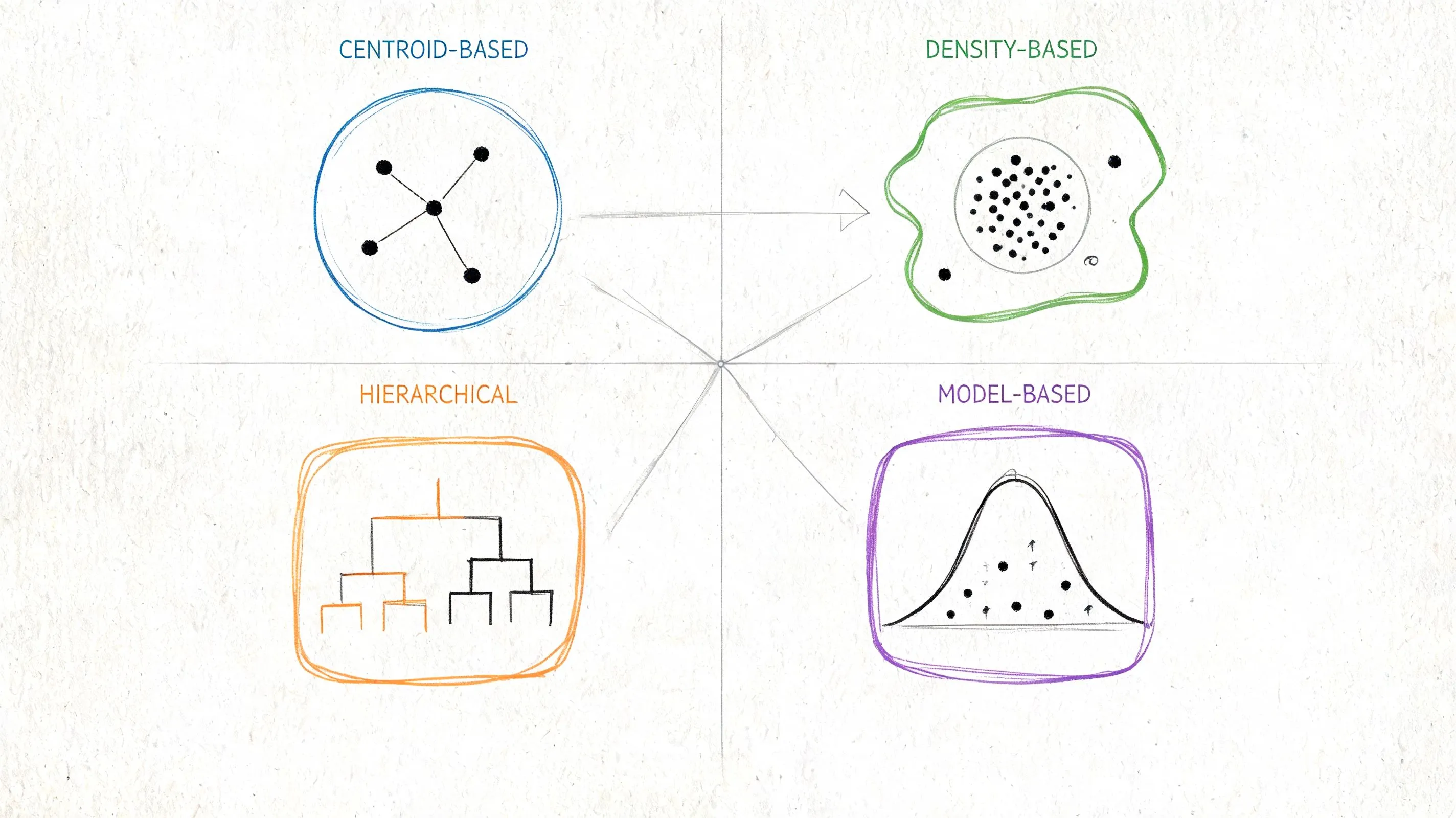
Before comparing named algorithms, it helps to think in families. Each family makes a different assumption about what a "cluster" is. That assumption determines where it works, where it breaks, and how much cleanup your team will need before trusting the output.

Partitioning methods

Partitioning algorithms divide data into a fixed set of groups. K-means is the best-known example, and it remains the most widely adopted clustering algorithm while also serving as a baseline for performance comparisons. Its staying power comes largely from computational efficiency, since k-means scales linearly with O(n) while many pairwise similarity methods scale with O(n²), which makes k-means practical for large datasets where less scalable methods become costly or impractical (research summary on clustering method scalability).

This family works well when you expect relatively compact groups and want something fast, simple, and easy to operationalize. That's one reason product teams reach for it first.

For teams developing machine learning judgment rather than applying a library default, this comprehensive guide for AWS ML professionals is a helpful companion, reinforcing the discipline of choosing methods based on system constraints rather than model familiarity.

Hierarchical methods

Hierarchical algorithms build nested groupings instead of one flat partition. In practice, Agglomerative Clustering starts with individual points and merges them upward into larger groups. The output is often a dendrogram, which can be useful when you care about relationships between segments, not just the final cut.

This family fits exploratory work well. If you're trying to understand whether "activated users" split into subtypes, a hierarchy can show that structure more naturally than a hard partition.

Hierarchical clustering is often easier to explain to stakeholders because it mirrors how people actually reason about segments. Broad groups first, finer distinctions second.

Density-based methods

Density-based algorithms define clusters as regions with enough nearby points. DBSCAN is the classic example. It doesn't require you to pre-specify the number of clusters, and it can discover irregular shapes while identifying points that don't belong anywhere obvious.

This matters in product data because not every user belongs to a clean segment. Some are edge cases, bots, one-time evaluators, or unusual enterprise admins whose behavior shouldn't pull the rest of the segmentation around.

Model-based methods

Model-based approaches assume the data was generated from underlying probability distributions. Gaussian Mixture Models, or GMMs, are the standard example. They're useful when you suspect overlap between groups and want softer assignment than "user X belongs only to segment Y."

These methods can be powerful when behavior is mixed. A user may partly resemble a light collaborator and partly resemble a high-value evaluator. A probabilistic model reflects that ambiguity better than a crisp partition.

How We Evaluated These Clustering Algorithms

In our review of clustering tools for product analytics, we judged each method against five criteria that matter in production: cluster shape assumptions, noise handling, scalability, parameter sensitivity, and fit for real workflows.

We focused on methods product teams run against event tables. That meant keeping K-means, DBSCAN, agglomerative clustering, Gaussian mixture models, and spectral clustering at the center. Methods like BIRCH or CANOPY were mentioned only briefly because they solve niche problems that rarely align with standard product data.

In practice, we found that parameter sensitivity is often the hidden killer. An algorithm that looks strong on a clean dataset can collapse when epsilon or min_samples is slightly off. That's why we weighted interpretability and rerun stability heavily — if a stakeholder can't understand why a user landed in a segment, the model fails its operational test even if the silhouette score is decent.

A Detailed Comparison of Common Clustering Algorithms

A product team usually asks a simple question: which clustering algorithm will give us segments we can ship, explain, and rerun next week without drama? That is the right question. In production, the choice is rarely about which method looks best in a textbook. It is about speed, tolerance for messy data, and whether the output survives contact with stakeholders.

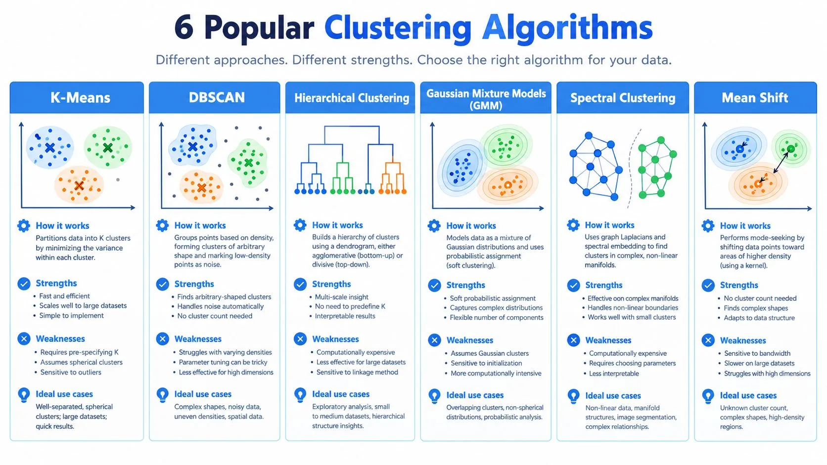
Clustering Algorithm Characteristics at a Glance

Algorithm	Scalability	Cluster Shape	Handles Noise/Outliers	Key Parameters	Best for	Fails when	What the output looks like in practice
K-means	High	Best for compact, centroid-like groups	Weak	Number of clusters	Fast segmentation of large, clean datasets	Irregular shapes or dense outlier clouds	Hard clusters, easy to visualize in dashboards
DBSCAN	Moderate, depends heavily on data and implementation	Arbitrary shapes	Strong, but sensitive to density variation	Neighborhood radius, minimum samples	Noisy data with varying densities	Very different densities across clusters	Dense regions clustered, oddballs labeled noise (-1)
Agglomerative Clustering	Lower on larger datasets	Flexible structure, depends on linkage choice	Moderate	Linkage, distance metric, cut level	Small to medium datasets needing interpretability	Large datasets with tight SLAs	Dendrogram, stable cuts at chosen levels
Gaussian Mixture Models	Moderate	Elliptical and overlapping groups	Weak to moderate	Number of components, covariance structure	Overlapping behavioral segments	Non-elliptical or sharply separated clusters	Soft probabilities per cluster, harder to explain
Spectral Clustering	Lower for large production datasets	Can capture complex boundaries	Moderate	Number of clusters, affinity settings	Subtle geometric structure in small data	Datasets growing beyond memory or compute

In our evaluation, a paper-backed snapshot of these trade-offs aligns with real-world usage. One comparative evaluation found that K-Means produced compact and well-separated clusters and was described as the most efficient method, while hierarchical clustering offered an interpretable dendrogram but scaled poorly, and DBSCAN handled arbitrary shapes and outliers but was sensitive to parameters — a split that still maps onto modern product analytics workflows (comparative evaluation of clustering methods).

Use the table as a screening tool, not a final decision. Teams working in self-serve analytics tools still need to inspect the output visually, because a decent metric can hide a segmentation that nobody can explain. If you are reviewing reduced features or cluster assignments, a scatter plot workflow for analytics teams is a fast way to check whether the model found structure or just imposed it.

Algorithm	Scalability	Cluster Shape	Handles Noise/Outliers	Key Parameters
K-means	High	Best for compact, centroid-like groups	Weak	Number of clusters
DBSCAN	Moderate, depends heavily on data and implementation	Arbitrary shapes	Strong, but sensitive to density variation	Neighborhood radius, minimum samples
Agglomerative Clustering	Lower on larger datasets	Flexible structure, depends on linkage choice	Moderate	Linkage, distance metric, cut level
Gaussian Mixture Models	Moderate	Elliptical and overlapping groups	Weak to moderate	Number of components, covariance structure
Spectral Clustering	Lower for large production datasets	Can capture complex boundaries	Moderate	Number of clusters, affinity settings

K-means

K-means remains the baseline many teams should try first. It is fast, widely supported, and easy to explain in product reviews. If the job is to split a large user base into a small number of broad behavior groups, K-means often gets you a usable first draft faster than anything else.

Its strength is operational simplicity. It scales well, retrains cleanly, and produces hard assignments that downstream teams can use in dashboards, alerts, and lifecycle campaigns. For a Querio-style workflow, that matters. Analysts can rerun it on fresh product tables without building a specialized pipeline.

It also fails in predictable ways.

• It assumes compact clusters. If your users form elongated, irregular, or nested groups, K-means will smooth those shapes into neat blobs.
• It assigns every point somewhere. Edge cases, bots, and one-off accounts still get forced into a segment.
• It is sensitive to outliers and feature scaling. Poor feature design can move centroids enough to make the segment story unstable.

A 2025 analysis of non-linear datasets showed DBSCAN outperforming K-means on concentric or irregular shapes, while K-means held up better on random point clouds because it partitions space more evenly (2025 analysis on non-linear datasets). Another health-risk profiling study reported DBSCAN achieving a silhouette score of 0.416 while K-means and hierarchical clustering scored around 0.045 to 0.046, underscoring how badly K-means can underperform when geometry matters.

K-means is best treated as a baseline with business value, not as a claim that the segmentation problem is solved.

DBSCAN

DBSCAN is often the better choice when product data is messy in ways teams already recognize. Fraud spikes, bot traffic, unusual enterprise admins, and one-time evaluators do not behave like clean centroid-based groups. DBSCAN can isolate dense pockets and leave genuine oddballs unassigned.

That changes the conversation with stakeholders. Instead of pretending every account belongs to a tidy segment, the model can say some accounts are noise. In production, that is often more honest and more useful.

Use DBSCAN when these conditions hold:

• Local neighborhoods are meaningful. Distances between points reflect real behavioral similarity.
• You expect outliers. Labeling noise is part of the job, not an inconvenience.
• Clusters may have irregular shapes. A single global centroid would blur the structure.

The trade-off is parameter tuning. Set the radius too small and one meaningful segment shatters into fragments. Set it too large and separate groups collapse together. DBSCAN also struggles when one part of the user base is dense and another is diffuse, which is common in product data with both power users and occasional users.

In practice, we found that epsilon and min_samples interact in non-obvious ways. Lowering epsilon without adjusting min_samples can explode the number of fragments, while raising min_samples can swallow small but real segments. A common fix is to explore parameter space on a sampled subset before committing to full runs.

Agglomerative clustering

Agglomerative clustering earns its keep when interpretability matters more than raw speed. It shows how records merge step by step, which gives analysts and product managers a structure they can inspect instead of a single fixed answer.

That is useful in account segmentation, customer research, and any workflow where the team wants to compare a coarse cut with a more detailed one. It also helps when the actual debate is not "which segment is correct" but "how granular should this segmentation be for action?"

Its practical strengths are straightforward:

• Good fit for small to medium datasets
• Useful for inspecting multiple cut levels
• Easier to defend in stakeholder discussions than many teams expect

Its main limitation is compute cost. As the dataset grows, rerunning agglomerative clustering can become slow and awkward, especially if analysts want to test several distance metrics and linkage choices. In a weekly production workflow, that overhead matters.

Gaussian mixture models

Gaussian Mixture Models are useful when hard boundaries are a poor description of reality. Many users sit between behaviors. A new admin can look like an evaluator early on, then shift toward operator behavior later. GMMs capture that overlap by assigning probabilities rather than forcing a single label immediately.

That flexibility comes with a communication cost. Probabilistic segments are harder to turn into a simple dashboard filter or a lifecycle rule. Data teams may appreciate the nuance, but product and marketing teams usually want a segment definition they can act on without reading posterior probabilities.

GMMs are a good fit when:

• Segments overlap materially
• You need soft assignment for scoring or ranking
• The data roughly follows elliptical group structure

They are less attractive when the team needs a crisp segmentation artifact for wide business use. In those cases, the model may be statistically better but operationally worse.

Spectral clustering

Spectral clustering can capture structure that simpler methods miss, especially when the boundary between groups is non-linear. On smaller datasets with subtle geometry, it can produce cleaner separation than K-means.

A comparative study of clustering performance across datasets found that results depend heavily on dataset size, dimensionality, and model order, and that no single method dominates across all settings (comparative study of clustering performance by size and dimensionality).

That finding matches production experience. Spectral clustering is often appealing during experimentation and less appealing during maintenance. It is harder to scale, more sensitive to affinity choices, and tougher to explain to non-technical stakeholders who need a reason a user landed in one segment rather than another.

K-means vs DBSCAN: the recurring choice

The most common question in our review was whether DBSCAN is better than k-means. The answer depends on your data shape and noise tolerance. If your users form compact, roughly spherical groups and you need speed, k-means wins on practicality. If you have uneven densities, outliers, or non-convex clusters, DBSCAN usually delivers segments that stakeholders can use.

A practical rule of thumb: start with K-means to establish a baseline, then switch to DBSCAN if the output forces noise into segments or misses elongated groups. In one evaluation of health-risk profiles, DBSCAN achieved a silhouette score of 0.416 while K-means scored only 0.045 to 0.046, illustrating when density-based methods dramatically outperform centroid-based ones on real-world data (2025 health-risk profiling study).

For most product teams, the practical decision framework looks like this:

• Start with K-means if speed and repeatability matter most.
• Use DBSCAN if outlier handling is part of the problem definition.
• Use Agglomerative clustering if interpretability and hierarchy matter.
• Use GMM if overlapping segments are real and useful.
• Use Spectral clustering when simpler methods clearly miss important structure and the dataset is still manageable.

How to Evaluate and Validate Your Clustering Results

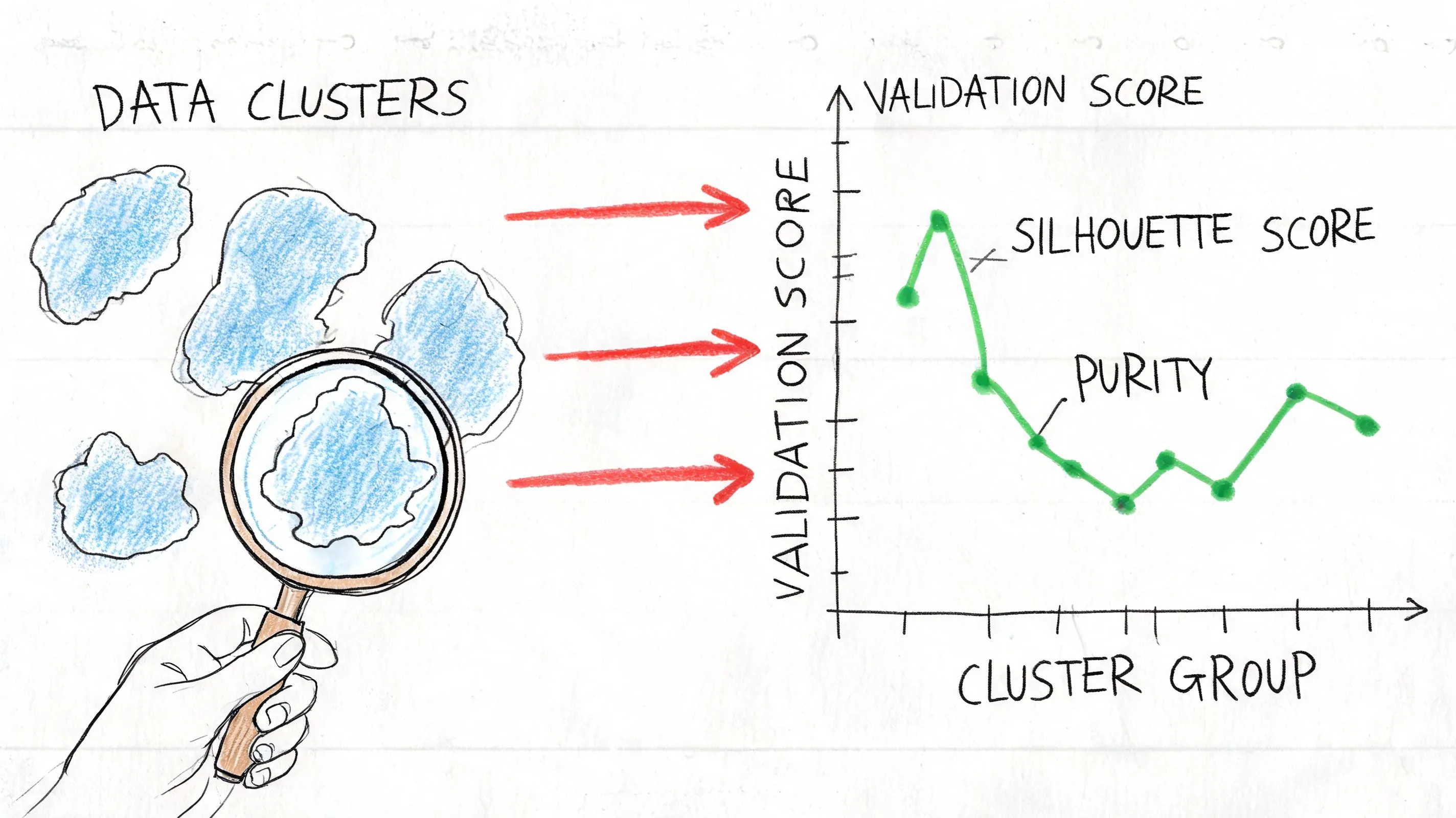
A clustering project usually fails after the model run, not during it. The team gets clean-looking segments, puts them in a dashboard, and then realizes nobody trusts them enough to act on them. Evaluation is the step that separates an interesting pattern from a segment your product, marketing, or success team will practically use.

Use metrics to reduce bad options early

Internal validation metrics are screening tools. They help teams rule out weak candidates before spending time naming clusters, wiring them into reports, or debating edge cases in a product review.

Silhouette Score, Davies-Bouldin Index, and Calinski-Harabasz Index remain the ideal initial collection for data science groups because they evaluate distinct failure modes. One identifies weak separation, another penalizes overlap, and another rewards compact structure. In practice, I look for agreement across metrics, not a single winning score.

Feature quality matters more than feature volume. Adding columns often makes clusters harder to interpret and less stable, especially in product data with redundant events, sparse attributes, and inconsistent tracking.

If your team needs a disciplined starting point, a basic exploratory data analysis workflow helps uncover skew, sparsity, and feature redundancy before you cluster anything.

A practical evaluation loop usually looks like this:

1. Run multiple algorithms on the same prepared feature set. Keep preprocessing fixed so the comparison is fair.
2. Compare internal metrics together. A model that looks good on one metric and weak on the others rarely holds up in production.
3. Inspect cluster sizes. Tiny shards or one oversized catch-all group often indicate that the algorithm is forcing structure onto noisy data.
4. Review feature distributions by cluster. The differences should be legible enough that a PM or analyst can summarize each segment without guesswork.
5. Test reruns. If small sampling or refresh changes produce different segment definitions, trust erodes fast.

One simple rule helps here. If the cluster description sounds like "users with medium values across many columns," the output is not ready for operational use.

Validate against decisions, not just scores

A high metric score does not make a cluster useful. The true test is whether the segmentation changes a decision with less friction.

Check whether the groups differ on outcomes your team already cares about, such as activation, retention risk, plan expansion, feature adoption, or support load. If those differences are weak, the clusters may still be mathematically tidy, but they will not earn a place in a self-serve analytics workflow.

This is also the point where teams should pressure-test interpretability. Ask product managers whether they can explain why a user belongs in a segment. Ask lifecycle marketers whether the segments support different messaging. Ask customer success whether the group definitions match what they see in accounts they manage every day.

A few checks work well in practice:

• Review clusters with domain teams. Product, marketing, and success teams often spot obvious nonsense quickly.
• Map clusters to actions. Every segment should suggest a report, campaign, experiment, or playbook.
• Check stability over time. Segments that swing after routine data refreshes create reporting churn and stakeholder skepticism.
• Document the preprocessing choices. Teams need to know whether scaling, dimensionality reduction, or outlier handling changed the result more than the algorithm itself.

For teams building this process with outside help, a good guide to machine learning consultancy is useful for understanding where external support adds value and where internal context matters more.

Good clustering survives three tests. It scores reasonably well, makes business sense, and stays stable enough that teams can use it week after week.

How to Choose the Right Algorithm for Your Product Data

A product team pulls a fresh user segmentation for a quarterly planning review. Marketing wants groups for messaging. Product wants behavior-based cohorts for roadmap decisions. Customer success wants accounts that need intervention. One clustering algorithm rarely serves all three jobs equally well.

Choose the algorithm based on the decision you need to support, the condition of the data, and the way the team will use the output week after week.

Start with the business use case

The first question is simple. What action will this clustering drive?

For campaign targeting, lifecycle messaging, or dashboards used by non-technical stakeholders, interpretability usually carries more weight than squeezing out a slightly better metric. K-means and Agglomerative Clustering are often the safer starting points because teams can describe the segments in plain language and revisit them without a long explanation.

For anomaly detection or edge-case discovery, density-based methods deserve more attention. DBSCAN can separate unusual records from the main population without forcing every user into a neat segment.

For experimentation or product behavior analysis, overlap may be part of the reality. GMM is useful when users sit between patterns, such as partially activated accounts that look like both new adopters and mature users.

Match the algorithm to the data you actually have

Algorithm choice depends heavily on dataset shape, size, feature quality, and noise. In production work, those factors matter more than textbook summaries.

A practical pattern works well:

• Large, fairly structured datasets: start with K-means or Mini-Batch K-means
• Smaller datasets where hierarchy matters: test Agglomerative Clustering
• Noisy data with outliers or uneven cluster shapes: test DBSCAN
• Behavioral overlap across groups: test GMM

This is a decision framework, not a contest.

Dataset size changes the shortlist quickly. Agglomerative methods can become expensive as the number of records grows. DBSCAN can also become hard to tune at scale, especially in high-dimensional product data. K-means remains popular in production for a reason. It is fast, easy to rerun, and usually good enough to establish a baseline before testing something more specialized.

Feature design matters just as much. Event-heavy product data is often sparse, skewed, and full of correlated signals. Before judging the algorithm, clean up the inputs. Scaling, transformations, and removing duplicate behavioral signals often change the result more than switching from one clustering family to another. Teams working through that step should review this guide to standardization in data workflows.

If your product data includes scraped web signals, a practical reference like WebscrapingHQ's page on mastering machine learning data collection can help align collection quality with downstream clustering readiness.

Choose for the operating model

A strong clustering result in a notebook can still fail in a real analytics workflow.

Teams need to rerun the segmentation after data refreshes, explain it to stakeholders, compare it with previous versions, and connect it to reports or campaigns. That requirement narrows the field. In self-serve environments like Querio, the best algorithm is often the one the team can reproduce and defend without relying on the original analyst every time.

That usually leads to a smaller production shortlist:

• K-means for speed, repeatability, and easy stakeholder communication
• Agglomerative Clustering when the hierarchy itself helps explain the groups
• DBSCAN when identifying noise and outliers matters as much as finding clusters
• GMM when hard boundaries would hide useful behavioral nuance

Teams should also be honest about tuning cost. DBSCAN and GMM can produce better segmentations for the right data, but they usually demand more parameter testing and closer review. If the team needs a segmentation that can be refreshed often by analysts, PMs, or operations staff, simpler methods often hold up better.

For organizations deciding whether to build this capability internally or bring in outside help, this guide to machine learning consultancy is a useful read because it frames the trade-offs between expertise, delivery speed, and long-term maintainability.

The practical mistake is treating algorithm choice as a one-time modeling decision. It is a workflow decision. Pick the method that fits the business question, survives the messiness of your product data, and remains usable after the first analysis is over.

Understanding Noise in HDBSCAN: What Labels -1 Mean

In HDBSCAN, the label -1 is reserved for noise. When a point receives that label, it means the algorithm did not assign it to any stable cluster under the chosen density hierarchy. That is not a bug — it is the intended behavior.

HDBSCAN extends DBSCAN by building a hierarchy of clusters at multiple density levels and extracting the most stable ones. Points that never fall inside a sufficiently stable region are flagged as noise. This is valuable because it prevents the model from forcing edge cases, bots, or rare accounts into a segment where they do not belong.

In practice, a high rate of -1 labels is usually a signal worth investigating. It can mean:

• Density variation is extreme. Some user groups are very tight while others are diffuse, and HDBSCAN is refusing to merge them artificially.
• Parameters are too conservative. A high min_cluster_size or tight core distance setting may reject clusters that are real but marginal.
• The feature space needs cleaning. Sparse, unscaled, or redundant features can distort distance calculations, making genuine users appear as outliers.

Compared to DBSCAN, HDBSCAN is often better at handling uneven densities because it searches across multiple epsilon values automatically. DBSCAN requires a single neighborhood radius, which means one global setting must balance both dense and sparse regions, a constraint that frequently fails in product data.

A practical example from product analytics: imagine you are segmenting app users by session length, feature breadth, and support tickets. Power users form a dense core. Casual users form a loose cloud. One-time evaluators and bots scatter far from both. Keeping those scattered points as label -1 lets you analyze the two main segments cleanly while reserving a separate "investigate" bucket for the noise. Forcing all of them into clusters would create a third segment that is too heterogeneous to act on.

When reviewing HDBSCAN output, always check the library documentation or implementation output, because integer cluster IDs typically reserve -1 for noise in common usage. If you are tuning, start by reducing min_cluster_size or inspecting the condensation tree to see where marginal clusters form.

From Theory to Practice on Querio

In practice, clustering projects fail less from algorithm choice than from workflow friction. The data is scattered across warehouse tables, feature definitions change midstream, and the person who needs the answer can't easily rerun the analysis.

A notebook workflow that works in practice

A sensible workflow starts with extracting user-level or account-level features from the warehouse. That usually means rolling event data into compact behavioral summaries such as sessions per week, feature breadth, activation lag, invite activity, or support-touch frequency.

From there, a notebook-based flow works well:

1. Profile the feature set first. Check missingness, skew, obvious outliers, and features that duplicate each other.
2. Create a baseline model. K-means is still a good starting point because it gives you a fast reference.
3. Test one structurally different alternative. If K-means is the baseline, compare it with something like Agglomerative Clustering or DBSCAN.
4. Review metrics and cluster profiles together. Numbers alone won't tell you which segmentation people will trust.

Teams that want to reduce manual warehouse-to-analysis handoffs can look at how AI-assisted analytics workflows replace manual data analysis, especially when repeatability matters as much as one-off exploration.

What teams should compare in one pass

A good experiment log should capture more than the algorithm name. Keep notes on:

• Feature set used
• Scaling choices
• Parameter settings
• Validation metrics
• Plain-English interpretation of each cluster

The important habit is comparison under controlled conditions. Change one thing at a time. If the features, scaling, and algorithm all shift together, nobody will know why the segmentation improved or degraded.

Frequently Asked Questions About Clustering Algorithms

How do I choose the number of clusters

Choose K based on decision value, not chart bends. For algorithms like K-means or GMM, start with a small range of candidate values and compare them using internal metrics plus business interpretability. Elbow plots can help, but they're often less decisive in real product data than people hope. Silhouette-based comparison is usually more useful when paired with manual inspection of cluster definitions.

A reasonable K selection workflow:

1. Run K = 3, 5, 7 with fixed preprocessing.
2. Compare silhouette scores across those runs.
3. Inspect cluster profiles for each K and ask whether stakeholders can distinguish the segments.
4. Pick the smallest K that produces actionable, stable groups.

Don't choose K just because the chart has a bend. Choose it because the resulting segments are distinct enough to support different actions.

When should I use OPTICS or HDBSCAN instead of DBSCAN

Use them when DBSCAN's single-radius assumption breaks. Plain DBSCAN can struggle when one cluster is tight and another is spread out. Methods like OPTICS and HDBSCAN relax that constraint by exploring reachability across multiple densities.

HDBSCAN is generally the stronger choice for product data because it extracts stable clusters from a density hierarchy and labels ambiguous points as noise (label -1) instead of forcing them into segments. OPTICS is useful for visualizing reachability plots during exploration, but HDBSCAN produces more directly operational labels.

If your team can't confidently tune either method, a well-parameterized DBSCAN often beats a fragile HDBSCAN run. Operational simplicity still matters.

What works better for noisy product data

No single algorithm is best overall — the best choice depends on cluster shape, noise, density variation, and operational needs.

For noisy product data, density-based methods usually outperform centroid-based ones. DBSCAN and HDBSCAN isolate outliers and handle irregular shapes, while K-means pulls noise into existing clusters and distorts segment boundaries. An overview of fuzzy and deep learning variants is available at this useful overview of clustering algorithms.

In one applied evaluation, DBSCAN achieved a silhouette score of 0.416 on health-risk profiling data, while K-means and hierarchical clustering both scored around 0.045 to 0.046, demonstrating how much centroid methods can underperform when noise and irregular geometry are present (health-risk profiling evaluation).

In plain terms:

• Use HDBSCAN when density varies widely and you want automatic noise labeling.
• Use DBSCAN when local density is consistent and you prefer a simpler, well-understood method.
• Use K-means only after strong preprocessing and when clusters are roughly compact.
• Use GMM when overlap is real and soft membership adds operational value.

If your data is noisy, don't force every user into a neat segment. Methods that can leave points unassigned or express partial membership often reflect reality better.

Querio helps teams run this kind of analysis directly on warehouse data with notebook-style workflows, so product managers, analysts, and data leaders can explore segmentation without waiting in an analytics queue. If you want faster, more flexible self-serve analysis, take a look at Querio.