Master the SUM Function in SQL Query

A founder opens a dashboard before the Monday leadership meeting and asks a simple question: “What’s our total revenue this month?” A product manager asks a different one: “How much engagement time did users generate after the new feature launch?” A finance lead wants one number for refunds, bookings, or payroll. Different teams, same pattern.

At the center of all those questions sits the sum function in SQL query work. Not the flashy part of analytics. Not the part people brag about. But the part that turns rows into a business answer.

If you’re early in your SQL journey, SUM() can look almost too simple to deserve much attention. Add a column. Get a total. Done. In production, it’s rarely that clean. Real tables have duplicates, missing values, awkward data types, expensive joins, and stakeholders who want totals broken down by channel, product, week, and customer segment.

That’s why this function matters so much. It’s one of the most impactful SQL skills you can build. Once you understand how SUM() behaves, how it interacts with GROUP BY, how windowed sums work, and where performance falls apart, you stop writing toy queries and start writing reporting logic people can trust.

If SQL still feels abstract, this primer on what databases are, why Excel breaks down, and where SQL fits is a helpful reset before you start thinking in aggregates.

Introduction Beyond Basic Arithmetic

A founder usually doesn’t ask for “an aggregate over a numeric column.” They ask, “What are we making?” That question sounds strategic, but the first technical step is often a sum.

Say you store subscription payments in a table called subscriptions. Each row has a customer_id, billing_month, and amount. To get monthly recurring revenue, you total amount. That’s SUM() doing the heavy lifting.

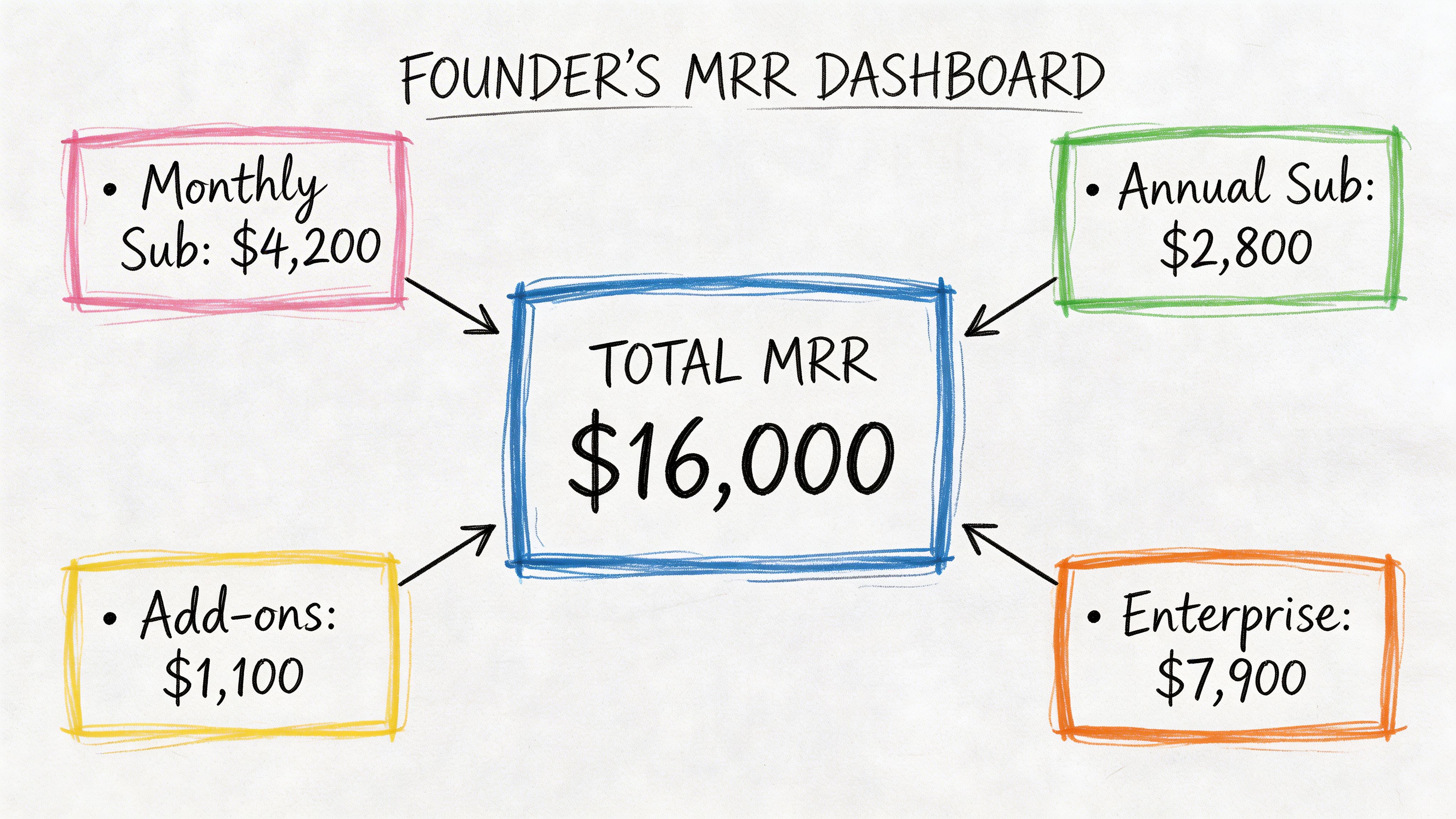
A product manager runs into the same pattern from another angle. Instead of revenue, they total minutes_watched, messages_sent, or credits_used. A support lead totals ticket handling time. An operations team totals units shipped. The business label changes. The SQL pattern doesn’t.

Here’s the basic shape:

SELECT SUM(amount) AS total_revenue
FROM subscriptions;

That query is short, but the answer can drive pricing decisions, hiring plans, and board updates.

Why this matters: Most dashboard metrics people call “KPIs” start as a sum, or as a formula built on top of one.

The gap between beginner SQL and production SQL starts right after this point. A junior analyst writes one total. A strong analyst asks better questions:

• Which rows belong in the total

• Are there duplicates

• Should nulls count as zero or be excluded

• Do we need totals by team, plan, country, or date

• Will this query still work when the table gets large

That’s where SUM() stops being arithmetic and becomes analytics infrastructure.

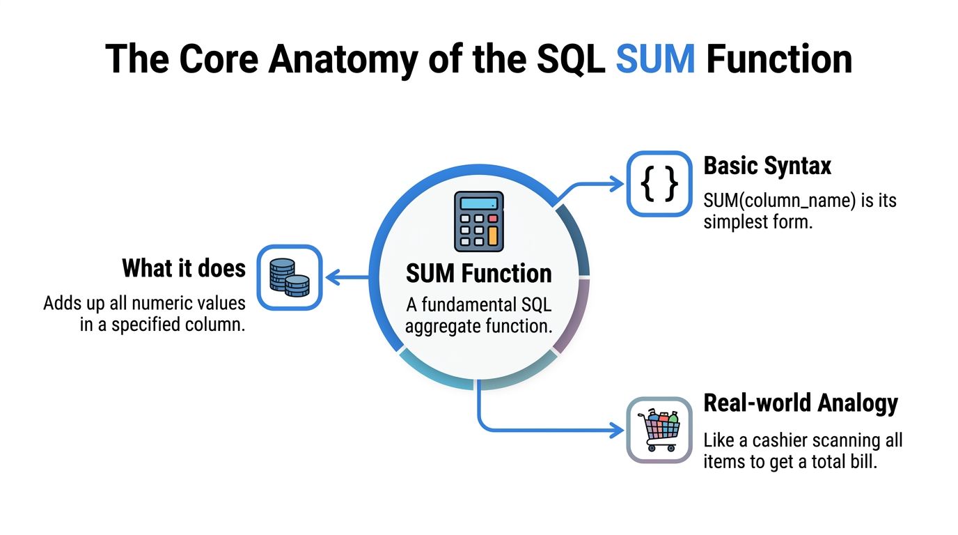
The Core Anatomy of the SQL SUM Function

SUM() is an aggregate function. It reads many row values and returns one total.

That sounds simple, but production use is rarely simple. A total can look correct even when a pipeline dropped rows, a column arrived as text, or a metric changed data type between warehouse layers. SUM() often sits at the center of revenue reports, usage dashboards, and finance checks, so small mistakes here spread fast.

If you want a broader foundation in everyday analytics patterns, this guide to the top SQL queries for analytics pairs well with the examples below.

Basic syntax

The basic pattern is short:

SELECT SUM(column_name)
FROM table_name;

Example:

SELECT SUM(quantity) AS total_units
FROM order_details;

SQL scans the quantity values and adds the numeric ones together. The result is one number for the full filtered dataset.

A good mental model is a warehouse audit. You are not inspecting each box one by one for its own sake. You are asking, "What is the total quantity across all boxes that made it into this table?"

What SUM can and can’t do

SUM() works on numeric data. Columns such as INT, BIGINT, DECIMAL, and FLOAT are valid, depending on your database.

It does not work cleanly on plain text categories like 'high', 'medium', or 'low'. It also becomes risky when numeric values arrive in string form because an ingestion job loaded '199.99' into a text column. Some engines fail immediately. Others try to convert values implicitly, which can create inconsistent results across environments.

In production, the safer approach is straightforward. Fix the type upstream if you control the pipeline. If you do not, cast explicitly in the query and document why you did it.

The NULL rule that trips people up

SUM() ignores NULL values. Oracle documents that behavior in its Oracle SUM documentation.

Example data:

Query:

SELECT SUM(session_minutes) AS total_minutes
FROM sessions;

Result: 50

SQL skips the missing value and adds the two known values.

That behavior is often correct for analytics. It is also a common way bad data slips through unnoticed. If NULL means "no session happened," skipping it makes sense. If NULL means "the event pipeline failed for part of the day," the total still returns a clean-looking number while the business metric is understated.

That is why experienced analysts do not stop at the total. They also check row counts, null rates, and load completeness. SUM() can hide gaps because it is designed to ignore missing numeric values, not explain why they are missing.

Why type behavior matters in production

Type behavior looks like a small implementation detail until the query powers a finance dashboard, a reverse ETL sync, or a self-serve metric that hundreds of people use.

Different databases can return different output types for the same SUM() expression. Even inside one platform, a sum over INT behaves differently from a sum over DECIMAL(18,2) or FLOAT. That affects precision, overflow risk, and how downstream tools display the result.

A few checks save a lot of cleanup later:

• Check the input type. Summing INT order counts is different from summing DECIMAL revenue.

• Check the output type. A currency metric usually needs fixed precision. A floating-point sum can introduce rounding surprises.

• Check the scale of the table. A column that fits safely today can overflow after months of growth.

• Check downstream consumers. BI tools, metric layers, and exports may format or cast the result again.

Here is a common production mistake. An analyst sums cents stored as INT, then another model divides by 100 and casts to a low-precision decimal for reporting. The number may look fine in a small sample but drift in large reconciliations because the cast happened too late or with the wrong precision.

A safer pattern is to be explicit:

SELECT SUM(CAST(amount AS DECIMAL(18,2))) AS total_amount
FROM payments;

That does not solve every database-specific edge case, but it makes your intent clear. Clear intent matters when a query gets reused in scheduled reports, data apps, or self-serve layers where other teams may never inspect the raw SQL.

SUM() is easy to write. Reliable totals require a little more discipline.

Grouping Totals with SUM and GROUP BY

A single grand total is useful once. After that, someone asks, “Can you break it down?”

That’s where GROUP BY changes the game.

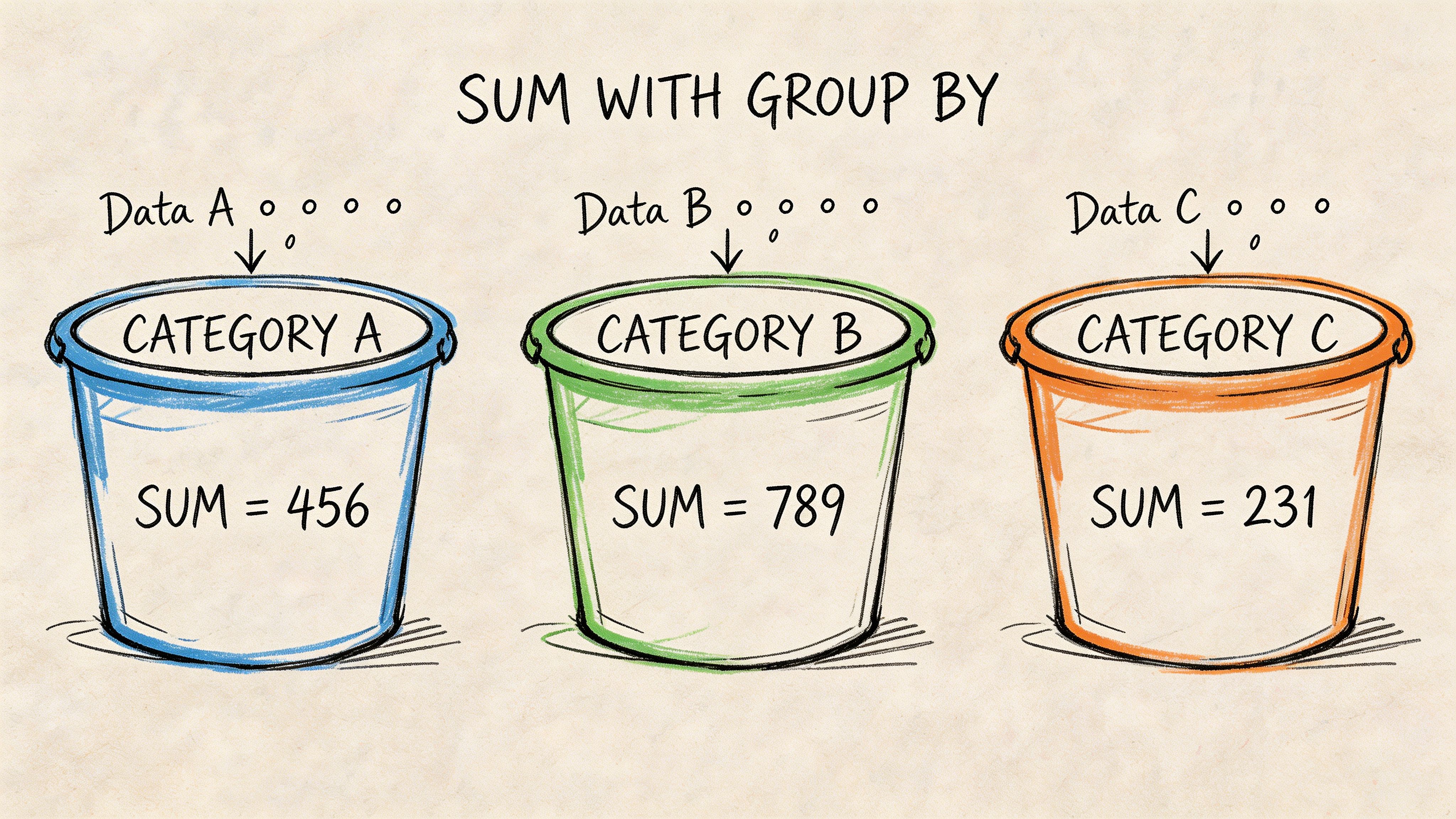
Instead of adding every row into one number, you tell SQL to create buckets first, then sum inside each bucket.

From one total to many subtotals

Suppose you have an order_details table:

A plain sum gives you all units across the whole table:

SELECT SUM(quantity) AS total_units
FROM order_details;

But most business questions need segmentation:

• Total units by category

• Revenue by campaign

• Credits used by workspace

• Refund amount by month

That’s what GROUP BY is for.

SELECT category, SUM(quantity) AS total_units
FROM order_details
GROUP BY category;

Result:

How to think about GROUP BY

The mental model is simple:

1. SQL reads the rows.

2. It groups rows with the same value together.

3. It runs the aggregate inside each group.

That’s why this pattern powers so many dashboards. You don’t just learn the total. You learn the shape of the total.

The SQL-92 standard brought SUM() and GROUP BY together as a common pattern, and one example cited in the verified material notes that SELECT OrderID, SUM(Quantity) FROM OrderDetails GROUP BY OrderID can segment data into 100+ groups while reducing query complexity by up to 70% versus equivalent procedural code, attributed there to Microsoft benchmarks via W3Schools’ SQL SUM reference.

The mistake people make most often

If you select a non-aggregated column, SQL usually expects that column in the GROUP BY.

This fails in many systems:

SELECT category, order_id, SUM(quantity)
FROM order_details
GROUP BY category;

Why? Because order_id is neither aggregated nor grouped. SQL doesn’t know which order_id to show for each category bucket.

Use this rule:

Practical rule: Every selected column must either be aggregated or included in the GROUP BY.

That one line saves a lot of debugging time.

A business example that shows the value

A marketing lead wants revenue by campaign. If each order row has campaign_name and amount, this query answers it directly:

SELECT campaign_name, SUM(amount) AS campaign_revenue
FROM orders
GROUP BY campaign_name;

That result becomes a dashboard table, a budget review, or a weekly growth meeting talking point.

If you want a quick visual walk-through before writing your own grouped totals, this short video is a useful companion:

Once you understand grouped sums, you’re no longer asking “What happened overall?” You’re asking “Where did it happen?”

Refining Aggregates with DISTINCT and Expressions

Basic sums answer broad questions. Production reporting usually needs more precision.

Sometimes the risk is double counting. Sometimes the challenge is that the metric doesn’t exist as a single stored column. You have to calculate it first.

When SUM DISTINCT helps

SUM(DISTINCT column) totals only unique values from that column. That’s useful when duplicate values would inflate the result.

Example:

SELECT SUM(DISTINCT discount_amount) AS total_unique_discount
FROM promotions;

If the same discount value appears repeatedly and your question is about unique values rather than every row occurrence, DISTINCT changes the result meaningfully.

This isn’t a default habit. It’s a deliberate choice. If duplicates are legitimate transactions, DISTINCT would undercount. If duplicates come from a messy join or repeated event rows, it may rescue the metric.

A good analyst asks first: “Are repeated values real activity or duplicate representation?”

Expressions inside SUM

A lot of useful business metrics aren’t stored directly.

Revenue is a classic example. You often have price and quantity, not revenue. So you compute row-level revenue inline, then sum it:

SELECT SUM(price * quantity) AS total_revenue
FROM order_items;

The verified material states that using expressions like SUM(Quantity * Price) requires the database to calculate the expression for each row before aggregating, and that SUM(DISTINCT col1) totals only unique values, which can reduce computational overhead for deduplicated metrics (GeeksforGeeks SQL SUM reference).

That detail matters more than it looks. The database isn’t summing a stored field. It’s doing row-by-row work first.

Combining logic before the sum

Real business rules often need conditional logic.

You may want:

• only paid invoices

• refunded revenue stored as negative amounts

• premium-plan usage separated from free-plan usage

That’s where conditional expressions become useful. If you want a quick refresher on writing branch logic inside SQL, this guide to the SQL CASE expression gives solid examples you can adapt.

A common pattern looks like this:

SELECT
  SUM(CASE WHEN plan_type = 'premium' THEN amount ELSE 0 END) AS premium_revenue
FROM invoices;

That query creates a selective total without filtering out the rest of the table.

Use expressions inside SUM() when the business metric is computed, not stored.

A quick decision check

Use plain SUM(column) when the column already represents the metric.

Use SUM(DISTINCT column) when duplicates would distort the meaning and you want unique values only.

Use SUM(expression) when you need to build the metric at query time.

Those three patterns cover a surprising amount of day-to-day analytics work.

Advanced Analytics with Window Functions and HAVING

Many SQL users advance from reporting to analysis.

A regular SUM() collapses rows into fewer rows. A windowed sum lets you keep the row detail while also calculating totals across a defined window. That’s how you build running revenue, cumulative signups, cohort progress, and trend lines without awkward self-joins.

If window functions still feel slippery, this practical guide to window functions in SQL is worth bookmarking alongside the examples below.

Running totals with SUM OVER

Suppose you have daily revenue:

A running total looks like this:

SELECT
  order_date,
  daily_revenue,
  SUM(daily_revenue) OVER (ORDER BY order_date) AS running_revenue
FROM daily_sales;

Result conceptually:

You still get each day’s row. You also get the cumulative total beside it.

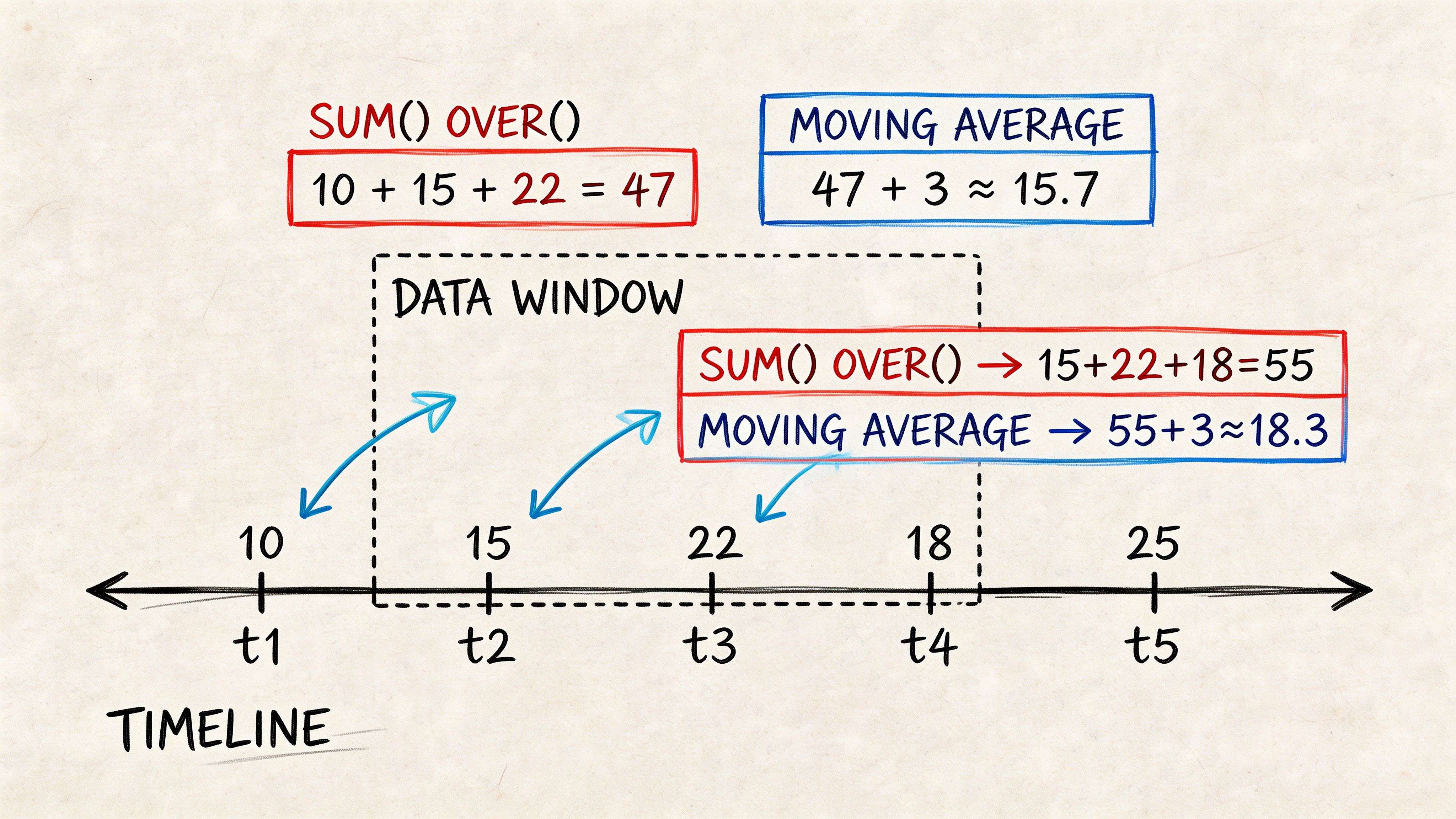
That’s a major difference from grouped aggregation. GROUP BY reduces detail. OVER() preserves it.

Why windowed sums matter in production

Window functions often replace repeated subqueries and messy joins. The verified material includes a future-dated claim that a 2026 dbt Labs benchmark found SUM() OVER() on Snowflake reduced query time by 65% compared with repeated subqueries for cumulative metrics, cited through the Microsoft SQL Server SUM documentation URL provided in the brief. Since that claim is future-dated in the materials, treat it as a benchmark note rather than a current universal rule.

Even without relying on that figure, the practical lesson holds. Window functions usually produce cleaner analytical SQL.

PARTITION BY for separate running totals

You can also calculate running totals within categories.

SELECT
  customer_id,
  order_date,
  amount,
  SUM(amount) OVER (
    PARTITION BY customer_id
    ORDER BY order_date
  ) AS customer_lifetime_spend
FROM orders;

Now each customer gets their own cumulative spend line.

That pattern is common in:

• Retention analysis

• Customer journey reporting

• Revenue expansion tracking

• Usage accumulation by account

HAVING filters after aggregation

HAVING works with grouped results. WHERE filters rows before grouping. HAVING filters groups after the sums are computed.

Example:

SELECT department, SUM(salary) AS total_salary
FROM employees
GROUP BY department
HAVING SUM(salary) > 500000;

That query asks: which departments have total salary above a threshold?

A row-level filter would use WHERE. A group-level filter uses HAVING.

Don’t use HAVING just because the condition mentions an aggregate. Use it because the decision depends on the aggregated result.

A useful mental split

If the question is “Which rows should enter the calculation?”, think WHERE.

If the question is “Which grouped results should survive after calculation?”, think HAVING.

That distinction sounds small. It changes both logic and performance.

Performance Gotchas and Production Best Practices

A sum query can look harmless in development and still become expensive in production. The usual pattern is familiar. A dashboard starts with one fact table, then picks up two joins, a few calculated fields, and a rolling total. The SQL still returns the right number. It just takes far more work for the warehouse to produce it.

Filter as close to the raw rows as possible

Row filters belong as early as possible in the query plan. Every row you remove before a join, sort, or aggregate is work the database no longer has to do.

That matters most on large fact tables. If you only need paid orders from the last 90 days, filter those rows before you sum revenue. If you wait until later, the engine may scan, join, and aggregate data you were never going to keep.

A simple mental model helps. SUM() is like adding items in a cart at checkout. WHERE decides which items even make it into the cart. Good production SQL keeps the cart small.

Use exact numeric types for money

Financial totals need predictable arithmetic. Floating-point types are built for range and speed, not exact decimal storage, so tiny rounding errors can surface when you sum thousands or millions of rows.

A concrete example makes this easier to spot. In IEEE 754 floating-point math, 0.1 + 0.2 can evaluate to 0.30000000000000004, which is fine for scientific data and a problem for revenue reporting.

For currency, teams usually cast to DECIMAL or NUMERIC before aggregating, or store the value in an exact type from the start. The database-specific syntax varies. The production rule does not.

SELECT SUM(CAST(amount AS DECIMAL(18,2))) AS total_revenue
FROM payments;

Watch the cost of per-row expressions

SUM(price * quantity) reads cleanly, but the database still has to compute price * quantity for every qualifying row before it can aggregate the result. On a small table, that cost is trivial. On a large event or order table, it can become one of the slowest parts of the query.

Three habits help keep that under control:

• Precompute stable metrics: If line-item revenue is reused across dashboards, calculate it upstream once instead of repeating it in every query.

• Reduce rows first: Apply selective filters before the expression runs.

• Standardize common logic: Put repeated revenue or margin formulas in models, views, or shared notebooks so analysts are not maintaining slightly different versions of the same metric.

That last point matters more as self-serve analytics grows. Once multiple teams are asking for the same totals, consistency becomes a production concern, not just a style preference. Querio, for example, runs AI coding agents directly on the warehouse and supports shared Python notebooks, which helps teams keep common query logic in one place instead of scattering copies across ad hoc reports.

Window functions can become the hidden bottleneck

Basic grouped sums are usually straightforward for modern warehouses. Windowed sums are where performance often starts to drift.

A running total such as SUM(amount) OVER (PARTITION BY customer_id ORDER BY order_date) requires the engine to partition, sort, and then compute across ordered rows. That is powerful, but it is also heavier than a plain grouped aggregate. If the partition key is high-cardinality, the sort keys are messy, or the query pulls more columns than needed, response time can climb quickly.

Two practical checks catch many problems:

• Select only the columns needed before the window calculation.

• Confirm the execution plan before rewriting SQL based on guesswork.

If a windowed sum feeds a dashboard that refreshes all day, it may belong in a summary table or materialized model instead of being recalculated from raw events every time. If you need a method for reading plans and trimming expensive steps, this guide to optimizing a query is a useful next step.

Correctness is only half the job

A production query has two responsibilities. Return the right number. Return it with a cost the business can afford.

Slow sums usually come from too many rows, repeated calculations, wide scans, or window operations that force large sorts.

That is where experienced analysts start. Check row counts after joins. Check whether a reusable metric should be modeled upstream. Check whether the same running total is being recomputed in every dashboard session. Those habits do more for production performance than clever syntax tweaks alone.

Conclusion From SUM to Self-Service Analytics

SUM() looks small because the syntax is small. The impact isn’t.

A founder checking revenue, a PM tracking engagement, and a data lead validating a finance model all rely on the same building block. First you learn the plain total. Then grouped totals. Then distinct handling, expressions, window functions, and post-aggregation filtering. After that, the focus shifts to reliability and speed.

That marks the turning point. They stop treating SQL as a bag of isolated tricks and start treating it as a way to encode business logic clearly.

The sum function in sql query work is also where self-serve analytics either succeeds or breaks. If totals are inconsistent, slow, or hard to explain, non-technical users lose trust fast. If the logic is standardized and the patterns are reusable, teams can answer routine questions without turning analysts into a human API.

That’s the broader shift worth aiming for. Analysts and data engineers should spend less time rebuilding the same totals and more time shaping the reporting layer, validating logic, and making the warehouse easier for everyone else to use.

If your team keeps getting stuck on repetitive reporting questions, Querio is worth a look. It puts AI coding agents directly on the data warehouse so teams can generate SQL, work in Python notebooks, and build self-serve analytics workflows without routing every aggregate question through an analyst.