A Practical Guide to Star Schema Data Modeling

A star schema is a straightforward way of arranging data in a warehouse. It’s built around a central fact table, which holds all your core business numbers (like sales totals or user sign-ups), and is connected to several dimension tables that provide the "who, what, when, and where" context. The whole thing looks like a star, which is how it gets its name.

This model is a favorite in business intelligence because it’s fast and incredibly intuitive to work with. Before we dig into why it’s so effective, let's quickly break down its two main parts.

Star Schema Components at a Glance

This table gives a quick summary of the roles that facts and dimensions play in the model. Think of it as your cheat sheet for understanding how the pieces fit together.

With this basic structure in mind, you can start to see how these simple components work together to make your data so much easier to analyze.

Why Your Analytics Need a Star Schema

Picture your company's raw data as a huge, disorganized library. When you need to answer a question, you're forced to rummage through thousands of unrelated books, trying to piece together information from different sources. That’s what it’s like running analytics directly on a transactional database—it’s slow, confusing, and a massive headache.

The star schema is the elegant fix for this chaos. It’s like a professional librarian who organizes everything with one goal in mind: fast, easy-to-understand analysis.

Instead of a tangled mess of tables, you get a clean, logical layout. You have one central "book" that contains the main story (your sales numbers, user activity, or other key events) and a handful of clear, concise reference guides that provide all the necessary background details—who the user was, what product they interacted with, and when and where it all happened.

The Foundation of Speed and Clarity

The real magic of the star schema is its simplicity, which is what makes it so fast. Developed by Ralph Kimball back in the 1990s, it was designed to overcome the sluggish performance of highly normalized databases that were great for daily operations but terrible for analysis. These older systems could require a dozen or more complex joins just to answer a basic business question.

The Kimball model, with its central fact table and surrounding dimensions, became the gold standard for data warehousing and analytics. It’s been shown to slash query times by up to 90% compared to traditional structures. In fact, over 70% of modern data warehouses still use a star schema approach, which is a powerful testament to its enduring value for self-serve analytics. For a deeper look at its history and structure, check out this overview of the star schema from OWOX.

This design delivers three critical benefits for any data-driven company:

• Blazing-Fast Queries: By drastically reducing the number of tables you need to join, queries run much, much faster. Dashboards load in seconds, not minutes, and you can get answers to spontaneous questions almost instantly.

• Intuitive for Everyone: The model is incredibly easy for both technical and non-technical people to understand. A business leader can look at a star schema diagram and immediately see the relationship between key metrics (facts) and their business context (dimensions).

• True Self-Service Analytics: This combination of speed and clarity is what makes modern BI and AI tools so powerful. When your data is in a well-designed star schema, product managers, founders, and marketers can explore data and find insights on their own, without waiting on the data team.

By simplifying the data landscape, the star schema turns the data warehouse from a complex repository that only engineers can navigate into an accessible resource that empowers the entire organization.

Ultimately, choosing a star schema isn’t just a technical decision—it’s a strategic one. It directly aligns your data infrastructure with the goal of making better, faster decisions. It's a cornerstone concept in data warehousing, a topic you can learn more about by reading up on the differences between a database, data warehouse, and data lake. Before we jump into how to build one, it's vital to appreciate why it remains the go-to model for so many successful companies.

Understanding the Core Components

So, what's really going on inside a star schema? To get a solid grasp on it, you have to understand its two main parts: a central fact table and all the dimension tables that connect to it. It’s a bit like reading a news story—the fact table gives you the headline numbers, while the dimensions fill in the crucial who, what, where, and when.

This separation is what makes the model so effective for business analysis. It neatly divides the raw, measurable events from all the descriptive context surrounding them. Let's break down each piece to see how they fit together.

Visually, it looks exactly like its name suggests: a central point with lines radiating outwards, forming a star.

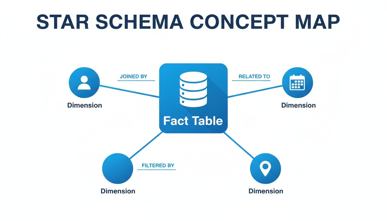
As you can see, the facts (the "what") are anchored in the middle, while the dimensions provide all the surrounding context that makes the data useful for analysis.

The Heart of the Model: The Fact Table

The fact table is the true center of your star schema's universe. This is where you store the core numerical metrics of your business processes—the raw numbers you want to add up, average, and track over time. These are the cold, hard "facts" of what’s happening.

Each row in a fact table represents a specific, measurable event. Since these tables log events as they occur, they tend to grow incredibly fast and often become the largest tables in a data warehouse, sometimes containing billions of rows. For a SaaS business, a fact table might log every user login, every subscription payment, or every feature interaction.

Fact tables aren't one-size-fits-all; they typically come in a few flavors:

• Transactional Facts: This is the most common type you’ll encounter. Each row is a snapshot of a single event at a single point in time, like a sale being completed or a support ticket being logged. A table named fct_user_logins is a classic example.

• Periodic Snapshot Facts: These tables give you a "picture" of performance at regular, set intervals. A fct_monthly_subscriptions table, for instance, would capture the total revenue and active users at the close of business each month.

• Accumulating Snapshot Facts: This type is built to track something as it moves through a defined workflow. A single row follows an entity, like a customer order, from start to finish. Columns get updated as the order hits key milestones, such as order_placed_date, shipped_date, and delivered_date.

The single most important concept for a fact table is its grain. The grain defines exactly what each row represents—for example, "one row per user login." Getting this right is absolutely critical for ensuring all your metrics are consistent and your calculations are accurate.

The Contextual Backbone: Dimension Tables

If fact tables tell you what happened, dimension tables are what tell you the who, what, where, when, and why. They are the descriptive tables that connect to your fact table and provide all the context you need to perform meaningful analysis.

Each dimension table is focused on a specific business concept, like dim_users, dim_products, or dim_geography. They are usually much smaller than fact tables and are filled with the attributes you’ll use to filter, group, and label your data. Your dim_users table, for example, would contain fields like user_name, signup_date, company_size, and region.

When it's time to run a report, you simply join these descriptive dimension tables to your numerical fact table. This is what allows you to "slice and dice" your metrics—for instance, joining fct_sales with dim_product and dim_geography to calculate total sales by product category in the North American market.

Since it was first formalized by Ralph Kimball back in 1996, the star schema has become the go-to approach for dimensional modeling. It's now used in over 75% of data warehouses because it makes reporting so much simpler. A transactional fact table might capture 100 million sales events a year, with metrics like revenue totaling $500M. This denormalized model, where dimensions provide the slicing power, has been shown to slash the need for custom SQL by up to 70% because built-in hierarchies (like Year > Quarter > Month in a time dimension) make drilling down a breeze. You can find more on its history on Wikipedia's page on the star schema.

By combining a central source of truth (the fact table) with rich, descriptive details (the dimension tables), the star schema gives you a foundation for business intelligence that is both intuitive and high-performing. If you're looking to build out your analytical stack, our business intelligence and data warehousing guide offers a much deeper dive into structuring your data for success.

Alright, enough theory. Let's get our hands dirty and actually build a star schema. This is where the concepts really click. I'll walk you through a proven, four-step process for designing a solid data model from the ground up.

Think of this as the framework we use to take messy, raw business data and transform it into something clean, fast, and genuinely useful for analysis. Get this part right, and you're setting your entire analytics platform up for success.

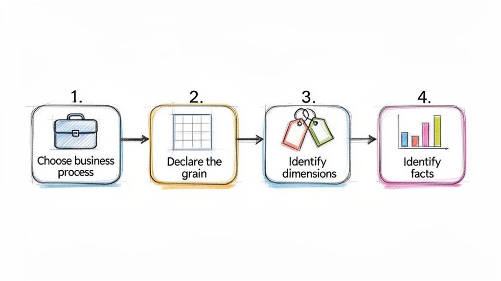
The Four-Step Design Process

Following a consistent method is everything. It helps you avoid common pitfalls and saves you from having to completely redesign your work months down the line. This approach, made famous by data warehouse pioneers like Ralph Kimball, is the industry standard for a reason.

1. Choose the Business Process: First things first, pick one specific business process to model. You can't boil the ocean, so focus on a single, well-defined area. Good examples include "user signups," "product sales," or "customer support tickets." We're looking for an activity that generates measurable events.

2. Declare the Grain: This is easily the most critical step, so don't rush it. You need to explicitly define what a single row in your fact table represents. This is the grain. Is it one order? One support call? Get specific. A great grain statement sounds like, "one line item per customer order." This decision dictates the level of detail for your entire model.

3. Identify the Dimensions: Once you know the grain, ask yourself: what context do I need to describe this event? The answers become your dimensions. For our sales line item grain, we absolutely need to know who made the purchase (Customer), what they bought (Product), and when the transaction occurred (Date). These are your "who, what, when, where, and why."

4. Identify the Facts: Finally, what did we measure? Facts are the numbers associated with the event, defined at the grain we declared. For a sales line item, the obvious facts are quantitative metrics like quantity_sold, unit_price, and total_sale_amount.

Follow these four steps, and you'll end up with a logical model where the numbers (facts) are clearly framed by all the descriptive context (dimensions) needed for analysis.

Handling Historical Data with Slowly Changing Dimensions

Here’s a real-world problem: your business data isn't frozen in time. A customer moves to a new city, a product gets a new name, or a sales region is reorganized. How do you track these changes without messing up your historical reports?

The answer is a technique called Slowly Changing Dimensions (SCDs).

An SCD is a method for managing and tracking the history of your dimension attributes over time. Picking the right SCD type is crucial for making sure a report you run today matches one you ran six months ago, even if the underlying data has changed.

While there are several types, you'll run into three main ones most of the time:

• Type 1 (Overwrite): The simplest approach. You just replace the old value with the new one. This keeps no history, so it’s best reserved for fixing mistakes, like a typo in a customer's name.

• Type 2 (Add New Row): This is the gold standard for historical tracking. When an attribute changes, you add a brand-new row for that dimension record (like a specific customer) with all the updated info. We typically use start_date, end_date, and is_current columns to show which version of the record is active.

• Type 3 (Add New Column): Here, you add a new column to the table to hold the previous value. This can be useful for tracking a single, specific change—for instance, previous_sales_rep—but it's not a scalable solution for attributes that change often.

Choosing your SCD strategy involves a trade-off. Type 2 gives you a perfect historical record but makes your dimension tables larger. Type 1 is easy to implement but effectively erases the past.

The Strategic Trade-Off of Denormalization

One of the core principles that makes a star schema work so well is denormalization. If you come from a software engineering background, this might feel wrong at first. In a typical application database (OLTP), you go to great lengths to avoid repeating data. But for analytics, we do it on purpose.

Instead of creating separate tables for product_category and product_brand and joining them to your dim_product table (a "snowflake" approach), a star schema intentionally puts those attributes directly into the dim_product table.

Yes, this means the brand name "Apple" might be stored thousands of times across your dimension, but that redundancy is a strategic choice. It completely eliminates the need for extra, performance-killing joins at query time.

This simplification is the secret to a star schema's speed. Your queries only have to join the big, central fact table to a handful of dimension tables, not navigate a complex web of relationships. The tiny bit of extra storage cost is a bargain for the massive improvement in query performance and the simplicity it gives your analysts. If you're new to writing these queries, our SQL guide for BI and analytics is a perfect place to start.

Comparing Star Schema, Snowflake Schema, and 3NF

While the star schema is a fantastic standard for analytics, it's not the only way to model your data. To really make the right architectural call, you have to understand the two other big players: the snowflake schema and the third normal form (3NF).

Each of these models was designed for a different job, and picking the right one comes down to what you’re trying to accomplish. A star schema is built for speed and simplicity, but is that always what you need? Let's break down the trade-offs.

The Trade-Off Between Simplicity and Storage

The fundamental difference between these models is their approach to normalization—the process of organizing a database to reduce data redundancy.

• A star schema is intentionally denormalized. It repeats information (like a category name) across many rows in a dimension table. This feels wrong at first, but it eliminates extra table joins, making queries run much faster.

• A snowflake schema is partially normalized. It takes a star schema's dimensions and breaks them out further. For example, a dim_product table might link to separate dim_category and dim_brand tables instead of storing that information directly.

• Third Normal Form (3NF) is highly normalized. This is the classic structure for transactional databases (OLTP systems). Every piece of non-key information is stored in exactly one place to ensure data is always consistent, which is critical for processing transactions efficiently.

Think of it like this: a star schema is a one-page cheat sheet, a snowflake schema is a detailed chapter with footnotes, and 3NF is the entire reference library. You need the library to write the book, but you'd grab the cheat sheet to quickly find an answer.

Star Schema vs. Snowflake Schema

At a glance, a snowflake schema can seem like a tidier, more organized version of a star schema. By normalizing dimensions, it definitely saves on storage space. And if a piece of information changes—like a brand name—you only have to update it in one small table.

But this tidiness comes with a hefty price tag: query performance. Those extra tables bring back the very problem star schemas were designed to solve. Every query now forces the database to perform more joins to stitch the data back together, which almost always slows things down.

The snowflake schema trades query speed for storage efficiency. In an era of cheap cloud storage and incredibly powerful data warehouses, this is rarely a good trade-off for analytics. The performance hit from extra joins almost always outweighs the minor storage savings.

For the vast majority of BI and analytics work, the star schema's simple, flat structure strikes the perfect balance. Its raw speed and intuitive design make it the clear winner for self-serve analytics, where business users need to explore data without becoming SQL experts.

Why 3NF Is a Bottleneck for Analytics

The single biggest mistake a growing company can make is pointing its analytics tools directly at a production database running in 3NF. While that 3NF structure is perfect for the application—processing orders, managing user accounts, and ensuring data integrity—it's a complete disaster for analytical queries.

Imagine asking a simple business question like, "Show me monthly sales by product category." In a complex 3NF model, that query could easily require joining a dozen or more tables. This puts an immense strain on the production database, slowing down the application for your actual customers and making the analyst wait forever for their results.

This is precisely why we build data warehouses in the first place. We extract data from the 3NF operational system, clean it up, and remodel it into a star schema that's optimized for the lightning-fast, read-heavy queries that analytics demands. This separation protects the app's performance and gives the data team a structure truly built for speed.

Model Comparison Star vs Snowflake vs 3NF

When you’re deciding on a data modeling strategy, it helps to see the strengths and weaknesses of each approach laid out side-by-side. The table below summarizes the key differences between a star schema, a snowflake schema, and a third-normal-form (3NF) model.

As you can see, there's a clear winner for most analytics use cases. While 3NF is essential for operational systems and snowflake schemas have their niche, the star schema's focus on query speed and simplicity makes it the undisputed champion for data warehousing and business intelligence.

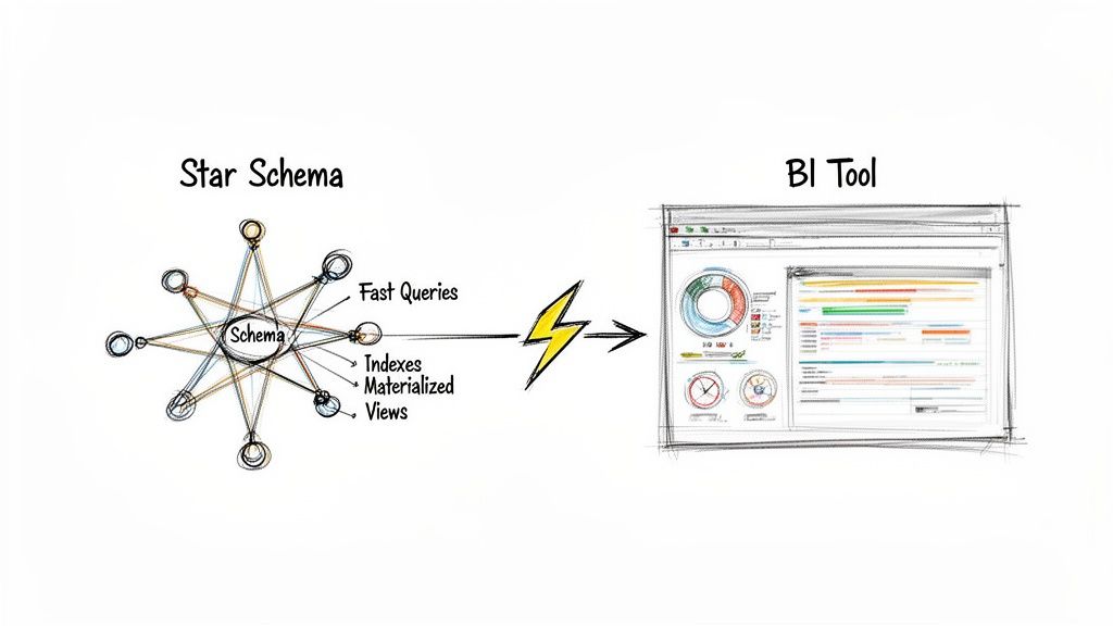
How Star Schemas Supercharge BI and Self-Serve Analytics

A well-designed star schema is what makes your data truly useful. Think of it as the high-performance engine for your analytics. When you connect a business intelligence (BI) tool like Tableau or Power BI to a star schema, you’re giving it a direct line to fast, clear, and intuitive data. This is where the hard work of data modeling pays off in real business value.

The most immediate impact? A massive boost in query speed. Instead of staring at a loading screen for minutes, users get answers in seconds. This isn't a small perk—it's the very thing that makes genuine self-serve analytics possible.

From Bottleneck to Empowerment

Without a star schema, non-technical team members often find themselves stuck, completely dependent on the data team for every little question. Each request becomes another ticket in a long backlog, killing momentum. The star schema flips this dynamic on its head by making the data model intuitive.

Suddenly, a product manager can explore a complex cohort analysis or a marketer can build a sales funnel, all with a simple drag-and-drop interface. They don’t have to know anything about complex SQL joins; the BI tool handles it all because the schema’s relationships are so clean and simple. This freedom lets them answer their own questions and iterate on ideas without waiting around.

The performance jump is hard to overstate. A star schema slashes query response times, which is a game-changer for startups that need to move fast. For example, a single business query might require 10-20 joins against a standard operational database. With a star schema, that number drops to just 4-5.

To put that in perspective, a query for 'monthly sales by region' on a fact table with a billion rows can run in under 2 seconds on a star schema. That same query on a traditional model could easily take over 5 minutes. Early benchmarks showed this structure could boost BI tool performance by 5-10x.

For those looking to master building these kinds of high-performance data solutions, the Microsoft Fabric Data Engineer Associate study guide is a great resource for practical, hands-on knowledge.

Technical Optimizations for Maximum Speed

While the star schema is naturally fast, data engineers can apply a few extra tricks to make it absolutely fly. These techniques are the secret sauce that delivers near-instant query results.

• Strategic Indexing: Think of an index like the index in a book—it helps the database find what it needs without reading every page. By placing indexes on the foreign keys in the fact table and the primary keys in the dimensions, we give joins a massive speed boost.

• Materialized Views: For common, complex queries that get run over and over, you can essentially "pre-calculate" the results and store them in a materialized view. When a user runs that query, the database just serves up the ready-made answer, delivering sub-second responses even on huge datasets.

• Partitioning: We can physically break up enormous fact tables into smaller chunks based on date (like by month or year). When a query asks for data from a specific time period, the database only has to scan that small partition, not the entire multi-billion-row table.

It’s these kinds of optimizations that make the star schema a resilient and scalable choice for any growing business.

By combining a simple, intuitive structure with targeted technical optimizations, the star schema transforms the data warehouse from a slow, cumbersome archive into a high-performance engine for decision-making.

Fueling the Next Generation of AI Analytics

The benefits don't stop with traditional BI dashboards. Today's AI-powered analytics platforms are built to thrive on well-structured data. For users on a platform like Querio, this means AI agents can query a star schema directly to get instant, conversational answers.

This setup allows a founder or product leader to ask about customer cohorts or track feature adoption in plain English, without ever opening a BI tool or writing a line of code. The star schema provides the clean, predictable foundation that AI needs to understand business context and deliver accurate insights.

It's what turns your data from a locked-away resource into an accessible, everyday tool for the entire organization. You can learn more about how this works in our article on semantic layers.

Common Questions About Star Schema Data Modeling

Once you start building star schemas, you'll inevitably run into some tricky situations. That's just part of the process. The world of data modeling is full of trade-offs, and knowing how to handle these common challenges is what separates a good model from a great one.

Let's walk through some of the questions that come up time and time again. Getting these answers right will help you build with confidence, whether you're navigating complex business rules or adapting to the speed of modern data.

Can I Use a Star Schema for Real-Time Data?

You absolutely can, but with a few important caveats. Star schemas are built for blazing-fast reads, not lightning-fast writes. The main challenge is getting fresh data in without bogging down the very analytical queries the model is designed to accelerate.

Modern data warehouses and streaming tools like Apache Kafka have made this much easier. They allow for micro-batching or even direct streaming into your fact tables. This gets you near-real-time data with a delay of just a few seconds or minutes, which is perfect for most business intelligence dashboards.

But what if you need true, sub-second reporting, like a live inventory count on an e-commerce site? For that, a transactional model (3NF) is usually the right tool for the job. A powerful and common pattern is a hybrid approach:

• Use a live OLTP system (transactional database) to run your daily operations.

• Continuously stream that data into a star schema for your analytics and BI.

This gives you the best of both worlds: rock-solid performance for operations and incredibly fast, flexible analytics.

How Does a Star Schema Handle Many-to-Many Relationships?

This is a classic modeling puzzle. A standard star schema loves simple one-to-many relationships—one product can be in many sales, one customer can make many purchases. But what happens when things get complicated? For example, how do you credit multiple salespeople for a single sale?

The answer is a clever little technique: the bridge table.

A bridge table is an intermediary table that sits between a fact and a dimension to resolve a many-to-many relationship. It breaks the complex link down into two simple one-to-many relationships.

Let’s stick with our sales example. To give credit to multiple salespeople for one sale, you’d set it up like this:

1. The Fact_Sales table holds the transaction details but instead of a salesperson key, it has a key pointing to the bridge table (e.g., Sales_Bridge_Key).

2. The Salesperson_Bridge table contains a separate row for each salesperson involved in that sale.

3. Each row in the bridge table then links to the Dim_Salesperson table.

This elegant solution keeps the star schema's simple structure and high performance intact while perfectly modeling your real-world business rules.

Is Denormalization in a Star Schema Bad Practice?

Not at all. In fact, it's a deliberate and essential design choice. This is what makes star schemas so fast and easy to use for analytics.

If your background is in software engineering or managing transactional databases (OLTP), the idea of duplicating data probably feels wrong. In those systems, normalization is critical for preventing errors during frequent writes and updates.

But in an analytical data warehouse, the game is completely different. We’re optimizing for read speed, not write efficiency. The "denormalization" in a star schema's dimension tables is a strategic trade-off. By placing descriptive attributes like product_category and product_brand directly into the Dim_Product table, we eliminate the need for extra joins at query time.

This intentional redundancy costs very little in terms of storage but pays massive dividends in query performance and simplicity. It’s the secret sauce that makes the model so intuitive for both BI tools and human analysts.

When Should I Choose a Star Schema Over a Snowflake Schema?

You should choose a star schema for over 90% of modern data warehousing needs. If your primary goals are fast query performance and ease of use, the star schema is almost always the right call. Its simple structure requires fewer joins, which makes queries run dramatically faster and the model far more intuitive for analysts to work with.

So, when would you ever use a snowflake? Only in very specific situations where you have massive, multi-level dimension tables and are under extreme storage constraints. For instance, a dimension with tens of millions of rows and deep hierarchies might be a candidate for "snowflaking" to save disk space. But this comes at a cost: you're trading that space saving for slower queries due to the extra joins.

In the era of cloud data warehouses, where storage is cheap and compute is powerful, the performance and simplicity of a star schema almost always win. For any team focused on moving fast and empowering users with data, it's the clear choice.

At Querio, we help you move beyond the limits of traditional BI by deploying AI agents directly on your star schemas. Our platform allows both technical and non-technical users to get instant answers from your data warehouse, turning your data team from a bottleneck into an enabler of self-serve analytics. See how you can scale your data insights at querio.ai.